Kai Foerster, University of Warwick, UK and Hertie School, Germany
Mobile money has been a key innovation in Africa that has increased the financial resilience of vulnerable households by providing an easy way to send and receive remittances. While recent literature has focused on the link between mobile money and its function as a social protection mechanism for the vulnerable population, less is known about the extent to which the costs of using the service affect the transaction behaviour of these people. By exploiting a natural experiment in the form of an excise fee that was imposed on mobile-money transactions in Kenya, this paper estimates the differential effect of a price hike in mobile-money transaction fees on transaction behaviour of households with a daily income below 1.25 USD and households above this threshold. The study finds that households with an income below 1.25 USD reduced their monthly mobile-money transactions volume by 25 per cent compared to households above this threshold. Additionally, the paper finds suggestive evidence that the tax also led to a relative reduction in mobile-money remittances received by households below an income of 1.25 USD. The loss in received remittances was not substituted by an increase in remittances sent by cash or in-kind.
Keywords: Mobile money in Kenya, financial resilience in developing countries, social protection mechanisms in developing countries, financial lives of the poor, excise duty on mobile money transactions, Kenyan Financial Diaries 2012/13
Mobile money has been a key innovation in Africa in the recent decade; it has been attributed to increased financial resilience of vulnerable households by providing an easy way to send and receive remittances (Jack and Suri, 2014; Riley, 2018). In Kenya, the first mobile-money service was launched in 2007 by Safaricom, a subsidiary of Vodafone (Jack and Suri, 2014). By 2013, 74 per cent of the Kenyan population above the age of 15 had a mobile-money account (Van Hove and Dubus, 2019).
Mobile money has reduced transaction costs, increased the geographical reach of financial transactions and guaranteed a speedy and safe arrival of money to recipients (Aron, 2018). Before the introduction of mobile money, sending money was a difficult and costly endeavour because fewer than 23 per cent of people had a bank account in Kenya in 2009 (Jack and Suri, 2011). For example, cash was sent through a trusted person or in-kind in the form of goods (Zollmann, 2014). In contrast, mobile money has enabled account holders to send each other digital values of money directly by way of text messages without the need for an internet connection. Apart from sending and receiving money, mobile money can be used to deposit and withdraw money at a mobile-money agent or to directly pay for goods (Van Hove and Dubus, 2019). Mobile-money operators fund their expenses by charging one-off fees for sending and withdrawing money. The charge varies between 0.2 per cent and 20 per cent of the transaction value according to the value and type of transaction (Safaricom, n.d.).
Buku and Meredith (2013) and Morawczynski (2009) explain that a key reason for the rapid expansion of mobile-money services in Kenya is the special socio-economic circumstance where a large share of urban workers send remittances back to their rural families who are more vulnerable to climate and weather-related shocks. Mobile money has enabled these vulnerable households to tap into a larger network of relatives and friends when requesting financial assistance to overcome sudden income shocks (Batista and Vicente, 2013; Blumenstock et al., 2016; Jack and Suri, 2014; Riley, 2018). Jack and Suri (2014) estimate that households receiving mobile-money remittances in Kenya were able to offset a drop in consumption resulting from negative income shocks, while households without mobile money suffered a consumption drop of 7 per cent on average. Riley (2018) finds very similar evidence for Tanzania.
By providing an easy and instant way to send and receive remittances, mobile money has been attributed to an increased financial resilience of many poor households in Kenya. To that respect, it has gathered momentum in the literature that attempts to establish a link between innovations such as (un)conditional cash transfers and micro-finance and their ability to function as social protection mechanism (Aron, 2018; Munyegera and Matsumoto, 2016).
A key difference between innovations such as (un)conditional cash transfers and micro-finance and mobile money is that remittances are sent through commercial mobile-money providers that charge transaction fees. Furthermore, the usage of mobile money requires both the sender and receiver to have access to a mobile phone and have the digital literacy to use the service. While recent literature has explored the extent to which digital literacy and access to a mobile phone limits the access of vulnerable populations to mobile money in developing countries, less is known about the extent to which transaction fees affect the transaction behaviour of vulnerable populations (Van Hove and Dubus, 2019; Wyche et al., 2016; Barasa and Lugo, 2015).
The introduction of an excise duty on mobile-money transactions in Kenya provides a natural experiment to study the differential effect that a price increase in transaction fees had on the transaction behaviour of vulnerable populations. On 1 February 2013, Kenya introduced a 10 per cent excise duty on fees charged by mobile-money operators to seek revenues from the rapidly expanding telecommunication sector (Matheson and Petit, 2017; Nord and Harris, 2013; Republic of Kenya, 2013a, 2013b). Safaricom, providing 70.7 per cent of all mobile-money accounts in Kenya, passed through the new duty fully onto customers on 8 February 2013, and they were followed by all other mobile-money operators in Kenya (Communication Authority of Kenya, 2014; Herbling, 2013; Safaricom, 2013).
The full pass-through of excise fees to customers de facto increased the fees customers had to pay to send mobile money over a short time frame. All else equal, economic intuition would suggest that customers might react to the price hike by reducing transactions. Moreover, economic intuition would also suggest that households with a tighter budget constraint might reduce transactions more than less constrained households because the price hike would weigh more into their budget relative to less constrained households.
To investigate whether the excise fee did disproportionately affect the transaction behaviour of more constrained, vulnerable households, this study applies a difference-in-differences estimation strategy to empirically estimate the effect the excise fee introduction had on transaction volumes and values for households with an income below 1.25 USD per person per day, in comparison with households with an income above this threshold. Such an estimation is possible thanks to high-frequency transaction data provided by FSD Kenya et al. (2015a, 2015b), which tracked 298 Kenyan households on a majority of their daily financial transactions between June 2012 and October 2013.
The paper finds that households below a daily income of 1.25 USD per person per day reduced their number of monthly mobile-money transactions by 25 per cent more than households above that threshold. Additionally, the paper finds suggestive evidence that the tax also led to a relative reduction in mobile-money remittances received by households with a daily income below 1.25USD per persons and that the loss of mobile-money remittances was not substituted by an increase in other modes of receiving remittances, such as by cash or in-kind.
The paper employs panel data of the Kenyan Financial Diaries from Digital Data Divide and Bankable Frontier Associates (FSD Kenya, 2014: 1). The survey tracked 298 households from June 2012 to October 2013 on 483,948 transactions (i.e. a vast majority of daily transactions made by these households). Additionally, the survey recorded socio-demographic characteristics of each household at the beginning of the survey (FSD Kenya, 2014: 1; Zollmann, 2014: 1-3). The fine-grained, high-frequency panel transaction data, including household-level socio-economic characteristics, provides an ideal starting point to investigate how the excise fee affected transaction behaviour of households with different characteristics.
The main drawback of the survey is that only about 1 per cent of the transactions (8334 transactions by 278 households) accounted for mobile-money transactions. Similarly, the survey picked up merely 1369 remittances made by mobile money and received by 183 households, 4332 remittances made by cash and received by 246 households, and 4681 remittances made in-kind and received by 229 households, which can be used for the analysis. It would have been best to analyse only households that were represented in all above categories so that relative comparisons between the categories was fully possible. However, this would have reduced the sample size even further. Given that the difference-in-differences estimator is an unbiased estimator and selection bias into remitting and transacting by mobile money is not the focus of analysis, the paper uses all above observations.
The above-mentioned observations are aggregated to the volume of monthly mobile-money transactions per household and the volume of monthly remittances received per household, broken down by whether they were received by mobile money, cash or in-kind. Furthermore, observations are also aggregated by the total monthly value of mobile-money transactions per household and the total values for remittances received broken down by mobile money, cash and in-kind transactions. For the main results, the paper focuses on the volume, rather than the total value, of transactions, given that the excise fee was levied on a unit – rather than value – basis. However, results are also discussed on the effect that the excise fee had on total monthly transaction values.
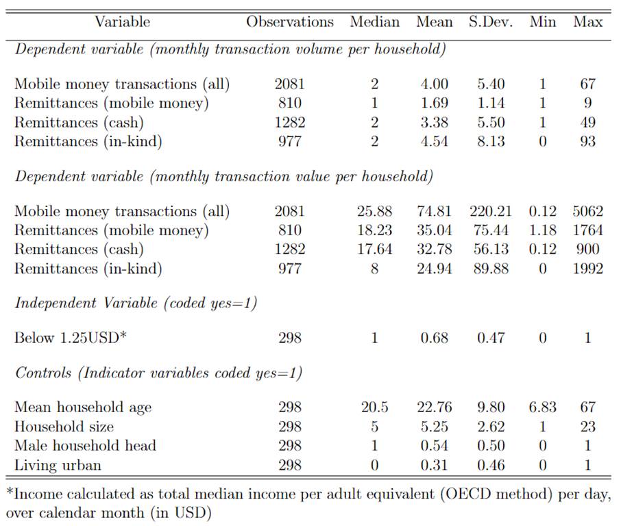
Table 1 illustrates summary statistics for the main dependent and independent variables. On average, households made approximately four mobile-money transactions per month, received approximately 1.7 remittances by mobile money, 3.4 remittances by cash and 4.5 remittances in-kind. These statistics are broadly in line with literature that suggests that households at the time made approximately four mobile-money transactions per month (Mbiti and Weil, 2011). In terms of total transaction values, households made mobile-money transactions worth approximately 75 USD per month. On average they received remittances via mobile money and cash worth 30–35 USD per month and in-kind remittances worth approximately 25 USD per month. It is noteworthy that all aggregate transaction measures are strongly skewed to the left, which is visible by the fact that the maximum value for each of the above variable is very large compared to the mean.
The key explanatory variable is the indicator variable ‘below 1.25USD’, which equals one if the income of the household calculated as total median income over a calendar month per adult equivalent (OECD method) per day was below 1.25 USD, and zero otherwise. Out of 298 households, 204 (68 per cent) in the survey made less than 1.25 USD per adult per day.
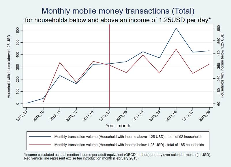
Figure 1 below gives a first intuition of how the monthly volume of mobile-money transactions was affected by the excise fee introduced in February 2013 (red vertical line). Households were grouped according to whether they made less or more than 1.25 USD, and the total volume of mobile-money transaction for each group was plotted. The figure documents that the volume of monthly mobile-money transactions of the group of households with an income below 1.25 USD and the volume of monthly mobile-money transactions of the group of households with an income above 1.25 USD were growing at a similar pace up until February 2013 when the tax was introduced. Thereafter, the volume of transactions of households below 1.25 USD income grew slower than that of households with a higher income, leading to a 10.9 per cent gap between the transaction volumes of the two groups by August 2013. This seems to suggest that the tax adversely affected the mobile-money transaction volume of households with a daily income below 1.25 USD relative to households with a higher income. All visual inspections remain intuition rather than causal evidence. Figures for monthly remittance volumes broken down by transaction method (i.e. mobile money, cash and in-kind) are provided in the Appendix.
This paper applies a difference-in-differences estimation strategy to estimate the causal impact that the 10 per cent excise fee had on the monthly mobile-money transaction volumes of households with an income below 1.25 USD per person per day.[1] The difference-in-differences estimator in this paper captures the difference between the actual monthly mobile-money transaction volume made by households with an income below 1.25 USD and the counterfactual transaction volumes these households would have made had the excise fee affected them as it affected households with an income above 1.25 USD per person per day. This gives an estimate of how much more households with an income below 1.25 USD were affected by the tax than households above this threshold. This estimator is also referred to as the average treatment effect (ATE) (Angrist and Pischke, 2009: 228).
The main difference-in-differences
regression model (referred to as main specification hereafter) which this paper
estimates by OLS is:

where mobile money transaction (vol)it is the monthly mobile-money transaction volume of household i in the month of year t (e.g. December 2012); below 1.25USDi is an indicator variable that equals one for households with an average income below 1.25 USD per day and is zero otherwise; Post taxt is an indicator variable equalling one if the data point is for an observation of monthly mobile-money transaction volume made after the excise fee introduction on 1 February 2013 and zero otherwise. The interaction term (below 1.25USDi X Post taxt)it equals one if the mobile-money transaction volume belongs to a household with an income below 1.25 USD after 1 February 2013. The coefficient estimate on the interaction term shows the differential growth in mobile-money transaction volume for households with an income below 1.25USD after the tax introduction compared to transaction volumes of all other households after the tax introduction. This coefficient size gives an estimate of the ATE. αi denotes the household-fixed effect, γt denotes the year-month fixed effect and ϵit is the error term. In line with Angrist and Pischke (2009) and Bertrand et al. (2004), standard errors are clustered at the household level to account for clustering and serial correlation in the error term.
For the ATE to be a causal effect, it is important that the monthly mobile-money transaction volumes of households with an income below and above 1.25 USD respond as similarly as possible to external factors, except for the policy of interest. In other words, the mobile-money transaction volumes of the households with an income below 1.25 USD and the transaction volumes of households with an income above that threshold should move parallelly to each other up until the excise fee is introduced. This condition is referred to as parallel trends assumption. Otherwise, the post-tax mobile-money transaction volumes of the households above the 1.25 USD threshold do not provide a good counterfactual to estimate the ATE because it will be difficult to believe that transaction volumes of households below 1.25 USD income would have grown at the same rate as those of households above the threshold had the tax not been implemented (Angrist and Pischke, 2009: 230).
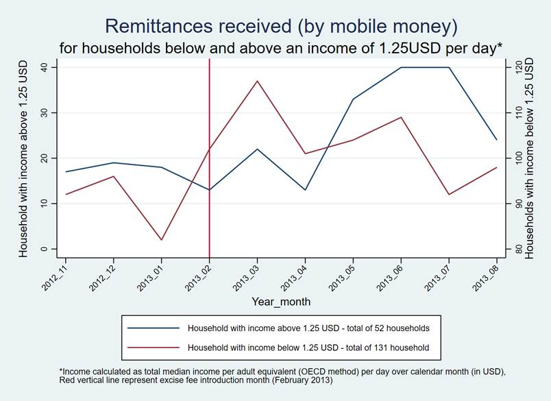
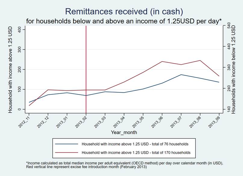
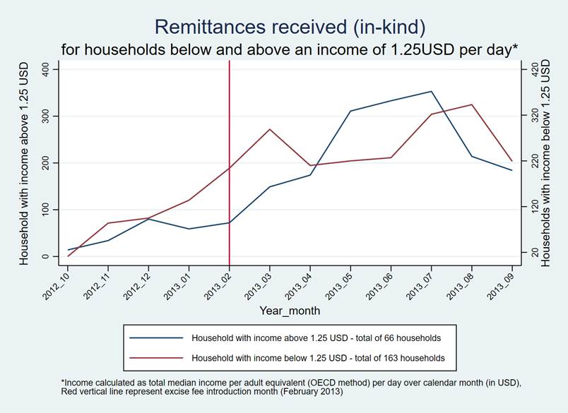
Figure 1 shows that the monthly transaction volumes of both groups move very similarly up to January 2013. After that, they diverge at the point where the tax was introduced. This shows strong visual evidence of parallel trends. Similarly, parallel trends are visible for monthly volumes of remittances received by cash (Figure 3 in Appendix) and partly also for remittances received in-kind (Figure 4 in Appendix) for the pre-treatment period. For monthly volumes of remittances received by mobile money (Figure 2 in Appendix), however, parallel trends are not visible. Therefore, the paper treats the OLS regression results using remittances as a dependent variable with caution.
To further investigate whether it is reasonable to assume parallel trends, in line with Clair and Cook (2015), a pre-treatment specification test and an event study is performed for mobile-money transaction volumes and values in Table 2 below and Figures 5 and 6 (Appendix), respectively. For all regression calculations, standard errors are clustered to the household level.
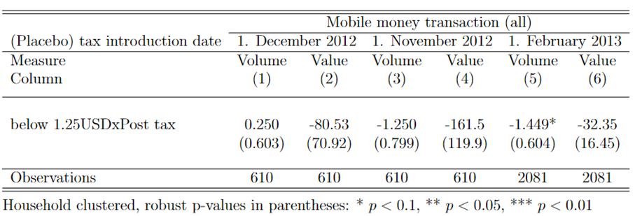
In Table 2, the main specification (Column 5) is compared against the regression results of the pre-treatment specification test. Column (1) runs the main specification, but Post tax is an indicator variable that equals one if the transaction was made after 1 December 2012, and is zero otherwise. Column (2) runs the same regression as Column (1), however Post tax is an indicator variable that equals one if the transaction was made after 1 November 2012, and zero otherwise. Furthermore, the sample size is restricted to observations made before the tax introduction between September 2012 and January 2013. By picking a tax introduction date that is prior to the actual date in a sample before the tax was introduced, Columns (1) and (2) function as a pre-treatment specification test that can pick up any diverging trends between the two household groups before the excise fee was introduced. The coefficient of interest is the coefficient on the interaction term of Post tax and below 1.25 USD income, which should be as close to zero as possible if poor and wealthy households were trending similarly pre-treatment. Indeed, for both Columns (1) and (2), the interaction term is far closer to zero than in the main specification and is statistically insignificant. In that respect, Table 2 provides further evidence that the volume and values of mobile-money transactions for both treatment groups were trending similarly before the tax introduction.
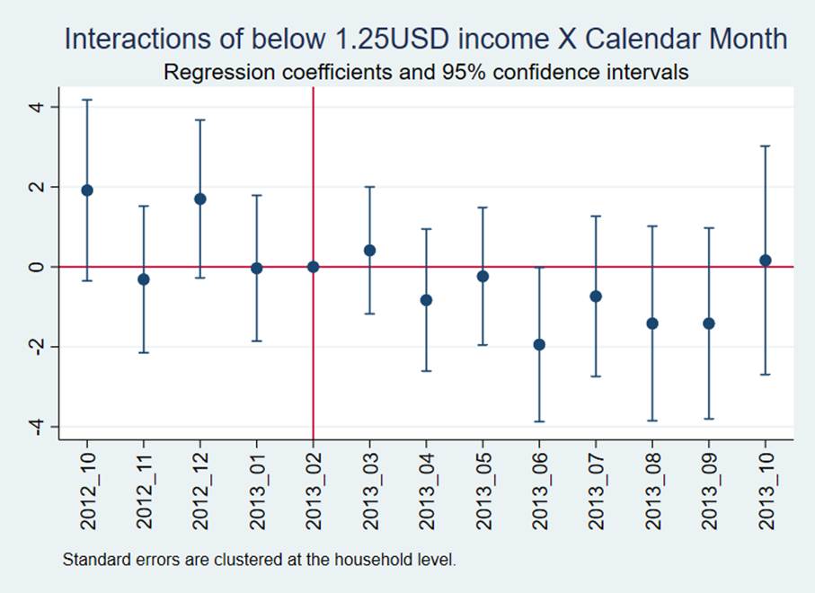
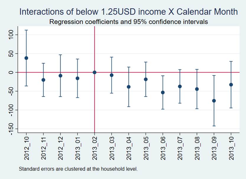
Further evidence for parallel trends comes from the event study in Figures 5 and 6 (Appendix). The event study plots the coefficient size and its 95 per cent confidence interval for the interaction between the indicator variable ‘below 1.25USD’ and every year-month observation. In Figure 5, the coefficients are plotted for mobile-money transaction volumes, and in Figure 6, they are plotted for total monthly values. The vertical line is present at February 2013, the month in which the excise fee was introduced. Both figures show that the coefficient sizes of the interaction terms were close to zero before the tax introduction and dropped to negative levels after the tax was introduced. This further provides evidence in favour of the parallel trends assumption. Furthermore, the drop in the size of the coefficient post-tax introduction indicates that the ATE estimate in the main specification is likely to be negative, confirming the economic intuition presented in the introduction section.
Table 3 shows the main results of this paper. For all results, standard errors are clustered to the household level. In Column (1), mobile-money transaction volumes is regressed on ‘below 1.25USD’. The coefficient on ‘below 1.25USD’ shows that households below 1.25 USD income make, on average, 2.6 mobile-money transactions per month fewer than households that have a higher income. This result is statistically significant at the 1 per cent level. In absolute terms, households with an income below 1.25USD made on average 2.8 transactions (see ‘Constant’–’below 1.25USD’) per month, while households with higher income made on average 5.4 transactions (see ‘Constant’), which is a large difference. One explanation for the usage difference is that poor households were less likely to own a mobile phone, which is essential for the usage of mobile money (Jack and Suri, 2011; Van Hove and Dubus, 2019). Mbiti and Weil (2011) estimate that mobile phone owners made three times as many mobile-money transactions as non-owners. Non-owners were far more likely to come from a low-income background (Aker and Mbiti, 2010).
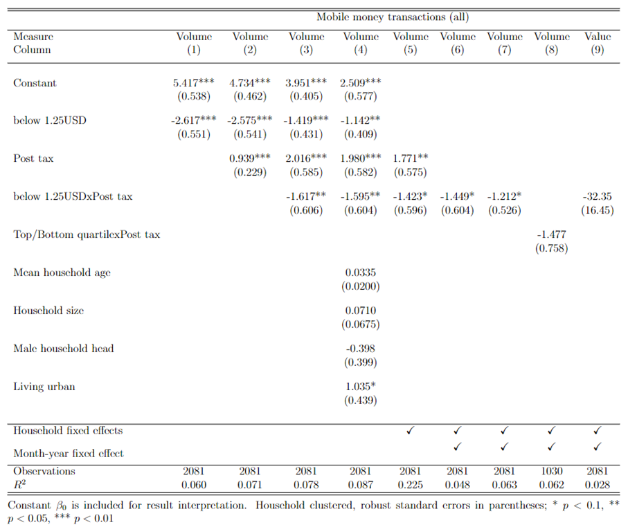
In Column (2), ‘Post tax’ is added to the regression. The coefficient on ‘Post tax’ shows that mobile-money transaction volume increased overall by an average of 0.9 transactions per month post-tax introduction. The result is statistically significant at a 1 level. These results are in line with the data from the Central Bank of Kenya, which shows that total mobile-money transaction volumes in Kenya increased from 53.5 million in February 2013 to 64.7 million by August 2013 (Central Bank of Kenya, n.d.). Herbling (2013) further suggests that the convenience of the service is a reason why Kenyans did not reduce their transaction volume despite the tax.
In Column (3), the interaction term between the ‘below 1.25USD’ and ‘Post tax’ is added. The coefficient on the interaction term suggests that post-excise-fee introduction, households with an income below 1.25USD reduced their transaction volumes by an average of 0.9 transactions compared to households above that income threshold. The result is statistically significant at a 5 per cent level.
Given that we found robust evidence for parallel trends, the interpretation of the coefficient on the interaction term can be extended. The result indicates that, while households with an income below 1.25 USD made, on average, 3.6 mobile-money transaction per month post tax, had they followed the counterfactual growth trajectory of households with a higher income, they would have made approximately 4.5 transactions per month. This is a reduction in monthly mobile-money transaction volume by 25 per cent compared to the counterfactual – a substantial drop. It suggests that the 10 per cent excise fee that increased transaction fees by the same size disproportionately affected households with an income below 1.25 USD. In line with the economic intuition presented in the introduction section, such behaviour may be explained through the more elastic demand of these households for mobile-money transactions due to their constrained budget compared to households with an income above 1.25 USD.
Columns (4)–(7) function as a robustness check for the estimates in Column (3). In line with Van Hove and Dubus (2019), Column (4) adds mean household age, household size, an indicator variable equalling one if the household head was male and an indicator variable that equals one if the household lives in an urban area as household-specific time-invariant control variables. This addition controls for potential household-specific characteristics that may bias the result in Column (3). Specifically, Riley (2018) and Van Hove and Dubus (2019) highlight that mobile-money usage differs on a village level – between rural and urban areas. The addition of the urban control variable addresses this potential omitted variable problem (Wooldridge, 2016). The size of the coefficient and the statistical significance for the interaction term change only slightly, suggesting that the coefficient is not driven by these household-specific factors.
In Column (5), household-fixed effects replace the control variables in Column (4). The reason for the usage of fixed effects is that they are able to account for any further time-invariant household-specific characteristic that may affect the transaction volume of mobile money (Wooldridge, 2009: 413).[2] The size of the coefficient and the statistical significance for the interaction term changes only slightly, suggesting that the coefficient is not driven by household-specific factors. This provides further evidence that the drop in transaction volumes for households with an income below 1.25 USD is due to the tax introduction.
In Column (6), a month–year fixed effect is added to the specification to account for possible common shocks over time at a national level. The addition does not affect the coefficient size and standard errors of the interaction term, suggesting that the estimate of the interaction term is also not driven by common shocks over time. Given that this specification is the most demanding in the sense that it accounts for all household-specific characteristics and common shocks over time, it is used as the main specification to which results from further robustness checks will be compared.
As mentioned in the data section, the transaction volume of mobile money is strongly left-skewed. Because the large values on the right tail can bias the OLS estimator (Wooldridge, 2009: 296), in Column (7), the main specification is rerun winsorising the top 1 per cent of mobile-money transaction volumes. The winsorising does not significantly alter the size and significance of the interaction term, providing further robustness to the results.
Another concern to the main specification is that the composition of household classified as ‘below 1.25USD’ could have changed over the course of the study period. For example, households that were just below the cut-off of 1.25USD on average, and were therefore classified as ‘below 1.25USD’, could have had a higher income post-tax introduction for an idiosyncratic reason and bias the results through their behaviour aligning more with the households with an income above 1.25 USD. To account for that, in Column (8), the main specification is run with households that are in the bottom quartile in terms of income calculated as total median income over a calendar month per adult equivalent (OECD method) compared with households in the top quartile. The alternative classification has the advantage of excluding the two quartiles in the middle of the income distribution. Given that it is less likely that any household in the top quartile would drop to the bottom quartile within the study period and vice versa, this specification is less prone to bias resulting from composition change. The size and significance of the interaction term stay relatively similar to the main specification, providing further robustness to the result.
Finally, in Column (9), the main specification is run with the monthly total mobile-money transaction values per household rather than monthly volumes of mobile-money transactions. While the coefficient on the interaction term is not statistically significant, the negative size of the coefficient is in line with the results of the main specification.
All in all, the robustness checks provide further evidence that the size and significance of the ATE estimate in the main specification are consistent.
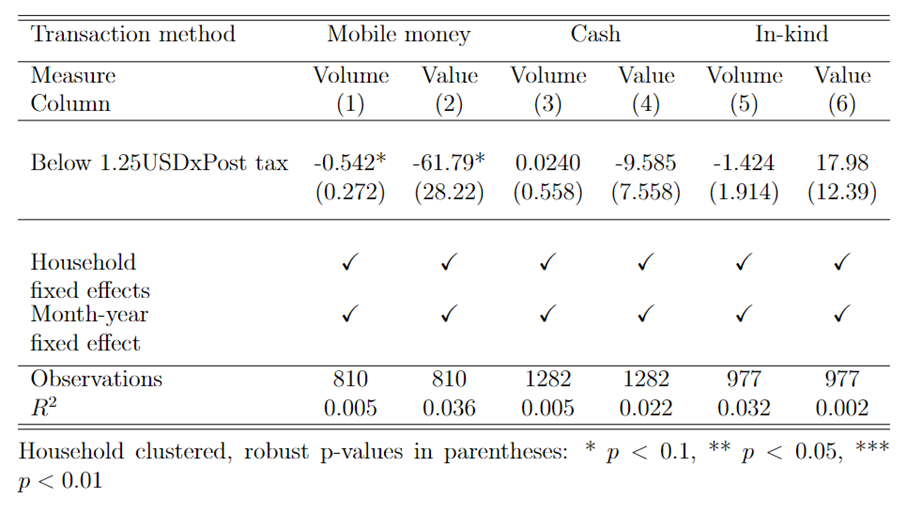
Table 4 turns to address the effect of the excise fee on the remittances. Remittances made by mobile money, cash and in-kind remittances made up 99.3 per cent of total remittances received by households in the survey, thereby capturing nearly the entire flow of remittances. By comparing the effect of the excise fee on remittances sent by mobile money with remittances sent by cash and in-kind, it is possible to grasp both the overall flow of remittances and the substitution between the transaction methods that the excise fee may have induced. It should be noted that results are only briefly discussed as they do not hold much explanatory power due to limited evidence in support for parallel trends.
Table 4 reports estimates from running the main specification for remittances received by mobile money (Columns (1) and (2)), cash (Columns (3) and (4)) and in-kind (Columns (5) and (6)) separately. In Column (1), (3) and (5), results in terms of volumes – that is, number of remittances received over a month – are reported, while Columns (2), (4) and (6) show results in terms of total value of remittances received over the specific months.
In Columns (1) and (2), the estimate of the interaction term is negative and statistically significant at a 10 per cent level. This suggests that the excise fee not only affected mobile-money transactions more generally, but also remittances sent via mobile money more specifically.
In contrast, there is little evidence suggesting that the excise fee impacted the volumes and total values of remittances received as cash and in-kind. There is no indicative evidence that households substituted remittances received by mobile money with cash or in-kind transactions as an alternative transaction method. However, this conclusion should be seen with caution as the sample size is smaller than for the main results and there is less evidence that the parallel trends assumption holds for remittances.
This paper has investigated whether the 10 per cent excise fee on mobile-money transactions levied in Kenya on 1 February 2013 disproportionately affected mobile-money transaction volumes of households below an income threshold of 1.25 USD per person a day. The study is the first of its kind to utilise a difference-in-differences estimation strategy to investigate the effect of a price hike in transaction fees on transaction behaviour of vulnerable populations in Kenya. The paper provides evidence that mobile-money transaction volumes of households with an income below 1.25 USD dropped by 25 per cent more than for households above the threshold. The study further indicates that these households would have made 25 per cent more transactions over the study period, had the excise fee not been introduced. Furthermore, the paper offers suggestive evidence that the excise fee also reduced remittances received via mobile money for households below an income of 1.25 USD compared to households with an income above this threshold. The reduction in remittances made by mobile money did not lead to a substitution with other transaction methods, indicating a potential slowdown in the growth of remittances flows to vulnerable households with an income below 1.25 USD compared to households with a higher income.
The findings of the paper highlight the importance of researching the extent to which the price of mobile-money transaction fees affects the transaction behaviour of vulnerable populations. This is because, for mobile money to function as a social protection mechanism, it must be accessible to the most vulnerable people. From a policy perspective, this study also provokes Kenya and other countries introducing mobile-money excise fees to rethink the benefits of such taxes with respect to the effect they might have on the social protection mechanism that the mobile-money service provides.
However, the above findings should also be interpreted with caution. One concern of the study is whether the ATE can be called a causal effect. As mentioned throughout the paper, evidence for parallel trends in some series was limited. Furthermore, it is noteworthy that the results attained in Kenya in 2013 might not apply to other countries and may also not apply to Kenya today as the economy transforms at a rapid pace.
Future studies could replicate the estimation using a control group of households outside of Kenya. With a larger sample size, it may be possible to analyse the flow of remittances with more statistical power and analyse the characteristics of those who send remittances and how they might change with the onset of the excise fee. Furthermore, the advantage of picking a control group outside of Kenya may be that the total effect of the tax on mobile-money usage could be estimated. Households from the CGAP Financial Diaries 2014–2015 (Anderson and Ahmed, 2016) – which tracked transactions of 86 households in Tanzania, a neighbouring country of Kenya, and 93 households in Mozambique, another East African country – may be a promising dataset to pick the control group from.
I would like to thank Dr Thomas Martin for his constant support and clear advice. I am also grateful to Dr Gianna Boero for valuable guidance during discussion on the research project.
Figure 1: Monthly mobile-money transaction volume for households with income above and below 1.25 USD over time
Figure 2: Monthly remittances volume (mobile money) for households with income above and below 1.25 USD over time
Figure 3: Monthly remittances volume (cash) for households with income above and below 1.25 USD over time
Figure 4: Monthly remittances volume (in-kind) for households with income above and below 1.25 USD over time
Figure 5: Event study using monthly mobile-money transaction volume
Figure 6: Event study using monthly mobile-money transaction value
Table 1: Summary Statistics
Table 2: Pre-treatment specification test
Table 3: Regression results – Impact of the excise fee on volume and total value of monthly mobile-money transactions
Table 4: Regression results – Impact of excise fee on remittances received
[1] The same methodology is applied to the analysis of remittances broken down by transaction method (mobile money, cash and in-kind).
[2] The Hausman test confirms the choice of a fixed effects over a random effects model.
Aker, J. C. and I. M. Mbiti (2010), ‘Mobile phones and economic development in Africa’, Journal of Economic Perspectives, 24 (3), 207–32
Anderson, J. and W. Ahmed, (2016), ‘Smallholder diaries. Building the evidence base with farming families in Mozambique, Tanzania and Pakistan’, Consultative Group to Assist the Poor (CGAP), available at https://www.cgap.org/sites/default/files/research_documents/perspectives_2_executivesummary.pdf
Angrist, J. D. and J. S. Pischke (2009), Mostly Harmless Econometrics – An empiricist’s companion, Princeton: Princeton University Press
Aron, J. (2018), ‘Mobile money and the economy: a review of the evidence’, The World Bank Research Observer, 33 (2), 135–88
Barasa, V. N. and C. Lugo, (2015). ‘Is M-PESA a model for financial inclusion and women empowerment in Kenya?’, in S. Moore (ed.), Contemporary Global Perspectives on Gender Economics, IGI Global, pp.101–23, available at https://doi.org/10.4018/978-1-4666-8611-3.ch006
Batista, C. and P. C. Vicente (2013), ‘Introducing mobile money in rural Mozambique: Evidence from a field experiment’, OVAFRICA Working Paper Series, 1303, 375–401
Bertrand, M., E. Duflo and S. Mullainathan (2004), ‘How much should we trust differences-in-differences estimates?’, The Quarterly Journal of Economics, 119 (1), 249–75
Blumenstock, J. E., N. Eagle and M. Fafchamps (2016), ‘Airtime transfers and mobile communications: Evidence in the aftermath of natural disasters’, Journal of Development Economics, 120, 157–81
Buku, M. W. and M. W. Meredith (2013), ‘Safaricom and M-Pesa in Kenya: Financial inclusion and financial integrity’, Washington Journal of Law, Technology Arts, 8 (3), 375–401
Central Bank of Kenya, (n.d.) ‘Mobile payments’, available at https://www.centralbank.go.ke/national%20payments-system/mobile-payments/, accessed 7 May 2020
Clair, T. S. and T. D. Cook (2015), ‘Difference-in-differences method in public finance’, National Tax Journal, 68 (2), 319–38
Communication Authority of Kenya (2014), ‘Quarterly sector statistic report – forth quarter of the financial year 2013/14’, Communication Authority of Kenya, 10, available at https://ca.go.ke/wp-content/uploads/2018/02/Q4SectorStatisticsReport2014-2013FINAL.pdf, accessed on 25 May 2021
FSD Kenya, Bankable Frontier Associates, Digital Data Divide (2014), ‘Kenya financial diaries 2012–2013 – data user guide’, available at http://s3-eu-central-1.amazonaws.com/fsd-circle/wp-content/uploads/2015/12/30093403/README-Financial-Diaries-Datasets-User-Guide-v1.1.pdf, accessed 25 May 2021
Herbling, D. (2013), ‘Mobile money transfers defy tax charge, rise to sh1.2 trillion’, Business Daily Africa, available at https://www.businessdailyafrica.com/Mobile-money transfers-shoot-up-despite-tax-/-/539552/2043490/-/e8k3siz/-/index.html, accessed 7 May 2020
Jack, W. and T. Suri (2011), ‘Mobile money: The economics of M-Pesa’, NBER Working Paper Series, 16721, available at http://www.nber.org/papers/w16721, accessed 7 May 2020
Jack, W. and T. Suri (2014), ‘Risk sharing and transaction costs: Evidence from Kenya’s mobile money revolution’, American Economic Review, 104 (1), 183–223
Matheson, T. and P. Petit (2017), ‘Taxing telecommunications in developing countries’, IMF Working Paper, 247
Mbiti, I. and D. N. Weil (2011), ‘Mobile banking: The impact of M-Pesa in Kenya’, NBER Working Paper Series, 17129
Morawczynski, O. (2009), ‘Exploring the usage and impact of “transformational” mobile financial services: the case of M-Pesa in Kenya’, Journal of Eastern African Studies, 3 (3), 509–25
Munyegera, G. K. and T. Matsumoto (2016), ‘Mobile money, remittances, and household welfare: Panel evidence from rural Uganda’, World Development, 79, 127–37
Nord, R. and E. Harris (2013), ‘Kenya: Fifth review under the three year arrangement under the extended credit facility and request for a waiver and modification of performance criteria’, IMF Country Report, (13), available at https://www.imf.org/external/pubs/ft/scr/2013/cr13107.pdf, accessed 7 May 2020
Republic of Kenya (2013a), ‘The Finance Act 2012’, Kenya Gazette Supplement, (221), available at http://kenyalaw.org/kl/fileadmin/pdfdownloads/Acts/Finance_Act_2012.pdf, accessed 25 May 2021
Republic of Kenya, (2013b), ‘The Finance Act 2013’, Kenya Gazette Supplement, 143, available at http://kenyalaw.org/kl/fileadmin/pdfdownloads/Acts/FinanceActNo38of2013.pdf, accessed 25 May 2021
Riley, E. (2018), ‘Mobile money and risk sharing against village shocks’, Journal of Development Economics, 135, 43–58
Safaricom (n.d.), ‘M-pesa rates’, available at https://www.safaricom.co.ke/personal/m-pesa/getting started/m-pesa-rates, accessed 7 May 2020
Safaricom (2013), ‘New government tax to hit 16 million M-Pesa users’, Safaricom PLC., available at https://www.safaricom.co.ke/about/media-center/publications/press releases/release/31, accessed on 7 May 2020
Van Hove, L. and A. Dubus (2019), ‘M-Pesa and financial inclusion in Kenya: Of paying comes saving?’, Sustainability, 11 (3), 568
Wooldridge, J. M. (2009), Introductory Econometrics – A modern approach, Princeton: Princeton University Press
Wooldridge, J. M. (2016), ‘What’s new in econometrics? Lecture 10: Difference-in-differences estimation’, National Bureau of Economic Research, available at http://www.nber.org/WNE/Slides7-31-07/slides˙10˙diffindiffs.pdf, accessed 7 May 2020
Wyche,S., N. Simiyu, and M.E. Othieno, (2016), ‘Mobile phones as amplifiers of social inequality among rural Kenyan women’, ACM Trans. Comput.-Hum. Interact, 23 (3)
Zollmann, J. (2014), ‘Kenya financial diaries – the financial lives of the poor’, FSD Kenya, available at https://www.findevgateway.org/sites/default/files/publications/files/kenya_financial_diaries_shilingi_kwa_shilingi_-_the_financial_lives_of_the_poor.pdf, accessed on 25 May 2021
FSD Kenya; Digital Divide Data; Bankable Frontier Associates, (2015a), ‘Kenyan Financial Diaries – All transactions’, Available at http://dx.doi.org/10.7910/DVN/JF8YST, Harvard Dataverse, V1
FSD Kenya; Digital Divide Data; Bankable Frontier Associates, (2015b), ‘Kenya Financial Diaries 2012-2013: Socio-economic and demographic datasets’, https://fsdkenya.org/dataset/kenya-financial-diaries-2012-2013-auxiliary-data/, FSD Kenya
Mobile money: Mobile money is a banking service that enables customers to send each other digital values of money directly by way of text messages without needing an internet connection. Apart from sending and receiving money, mobile money can be used to deposit and withdraw money at a mobile-money agent or to directly pay for goods.
Remittances: Informal financial assistance sent between close friends and family.
Excise fee: A tax that is levied on transaction fees charged by mobile-money providers.
Financial resilience: The ability to withstand income and consumption shocks and other forms of financially stressful events such as health problems.
Difference-in-differences estimation strategy: An econometric method that enables researchers to estimate causal effects between two variables of interest.
OLS regression: A statistical method that fits a statistical model as best as possible to the underlying data.
Vulnerable households/people/population: In the development economics literature, it refers to socio-economically disadvantaged people.
Natural experiment: A real world event that naturally split the population into a treated and untreated group in a quasi-random manner.
Pass-through: Passing on additional costs of providing a service / offering a product fully to the customer.
Winsorising: Recode the bottom/top x per cent of the cases in a variable to the values corresponding to the xth and the (100-x)th percentile.
Counterfactual: A thought exercise of how an outcome would have been had a condition been different. In empirical economic literature more specifically, it refers to an causal outcome that would have materialised had one specific condition been different.
Parallel trends assumption: The underlying assumption for the difference-in-difference estimation strategy to yield causal estimates. Visually speaking the assumption states that if two series move together over time, one can more reasonably believe that the series are affected by the external environment in the same way. Hence, when a new treatment shakes up the parallel trends, one can more reasonably argue that the shake-up is due to the treatment rather than over factors.
To cite this paper please use the following details: Foerster, K. (2022), 'Does Taxing Mobile Money Harm the Poor: Evidence From the 10 Per Cent Excise Fee Introduction in Kenya', Reinvention: an International Journal of Undergraduate Research, Volume 15, Issue 2, https://reinventionjournal.org/article/view/845. Date accessed [insert date]. If you cite this article or use it in any teaching or other related activities please let us know by e-mailing us at Reinventionjournal@warwick.ac.uk.