Preliminary Testing: The devil of statistics?

Jack Pearce and Ben Derrick, Applied Statistics Group, University of the West of England, Bristol

Abstract

In quantitative research, the selection of the most appropriate statistical test for the comparison of two independent samples can be problematic. There is a lack of consensus in the statistics community regarding the appropriate approach, particularly towards assessing assumptions of normality and equal variances. The lack of clarity in the appropriate strategy affects the reproducibility of results. Statistical packages performing different tests under the same name only adds to this issue.

The process of preliminary testing assumptions of a test using the sample data, before performing a test conditional upon the outcome of the preliminary test, is performed by some researchers; this practice is often criticised in the literature. Preliminary testing is typically performed at the arbitrary 5% significance level. In this paper, this process is reviewed and additional results are given using simulation, examining a procedure with normality and equal variance preliminary tests to compare two independent samples.

Keywords: Statistics, robustness, t-test, preliminary testing, conditional tests, independent samples

Introduction

In statistical hypothesis testing, the literature rarely reaches an agreement on the most appropriate analysis strategy for any given scenario. To illustrate the problems faced, this paper will focus on comparing the central location of two independent samples. For example, some researchers may use an independent samples t-test with pooled variances (Independent t-test), some may use a form of the independent samples t-test not constrained to equal variances (Welch's test), others may use the Mann-Whitney or the Yuen-Welch test due to concerns over normality.

Each of these two-sample tests has accompanying assumptions. The Independent t-test assumes both normality and equal variances. Welch's test assumes normality but not equal variances. The Mann-Whitney test assumes equal variances but not normality. Yuen-Welch's test has no assumptions regarding normality or equal variances.

Assessment of the assumptions to determine the appropriate two-sample test can occur either at the design stage or after the data has been collected in the form of preliminary tests of the assumptions. A researcher could have a plan to perform one of the above tests based on pre-existing knowledge of the assumptions, or they might plan to perform preliminary tests on the assumptions to determine the correct test, or they may have no plan at all.

There is no consensus as to the correct method of preliminary analyses, which results in researchers choosing tests in ad-hoc ways – even selecting methods of analysis after the data has been compiled that provides the desired conclusion. This has contributed to the reproducibility crisis in the sciences.

The Independent t-test is taught as the 'standard' two-sample test. Undergraduate students are taught how to run the test, but not necessarily the definitive set of conditions when it might be appropriate, or the knowledge to evaluate the appropriateness of the test. Along with many practical users, undergraduate students will follow a set of arbitrary instructions based on an arbitrary decision tree provided by their lecturer or other resource. Many decision trees outlining a two-sample test procedure can be found on the internet (Martz, 2017) but rarely in academic papers. One example of a two-sample test decision tree in an academic paper is Marusteri and Bacarea (2010), this involves both normality and equal variance preliminary tests.

Before an informed decision can be made as to whether the Independent t-test is the most appropriate two-sample test, questions regarding the assumptions of the Independent t-test must be answered, namely checking if the data is normally distributed and the group variances are equal. Preliminary tests can be used to answer these questions. However, there are many different tests that could be performed to check the assumptions. To check the normality assumption, the Shapiro-Wilk test or the Kolmogorov-Smirnov test could be performed, among others. The tests for equality of variances assumptions could be Levene's test using deviations from the group means or Levene's test using deviations from group medians, among others.

Another issue with regards to reproducibility is the fact that different software run different tests under the same name. For assessing equality of variances, SPSS runs Levene's test using deviations from means, whereas Minitab runs Levene's test using deviations from medians. This affects reproducibility, because both SPSS and Minitab are widely used statistical packages in quantitative research. Researchers may run what they believe is the same Levene's test for equal variances but receive conflicting conclusions, affecting their chosen conditional two-sample test and thus the final conclusions.

For example, in the following table, data has been collected from an exam consisting of 20 multiple-choice questions taken by two different tutorial groups, i.e. there are two independent samples. The scores awarded by the participants of the exam can be found in Table 1.

The decision rule applied by both SPSS and Minitab is: if the null hypothesis of equal variances is failed to be rejected, the Independent t-test is performed; conversely Welch's test is performed when variances are found to be unequal. If one researcher uses SPSS and the other uses Minitab, the following would occur, as per Table 2.

As seen in Table 2, testing at the 5% significance level, performing the procedure on SPSS with Levene's preliminary test (using means), the researcher would reject the assumption of equal variances (p = .030); the conditional test is therefore Welch's test, which finds no significant difference in the mean scores (p = .051). However, performing the procedure on Minitab with Levene's preliminary test (using medians), the researcher would fail to reject the assumption of equal variances (p = .071) and would then run the Independent t-test and find a significant difference in the mean exam scores (p = .046).

Therefore, two researchers with the same data would arrive at different conclusions simply due to the software used. Hence, even if there was a consensus as to the correct preliminary test procedure to run, researchers can have a hard time producing the same results. It is apparent that a lack of a plan and user apathy as to which statistical tests are being performed is dangerous. Moreover, a researcher could reverse engineer the software used and statistical test performed in order to achieve their desired conclusion.

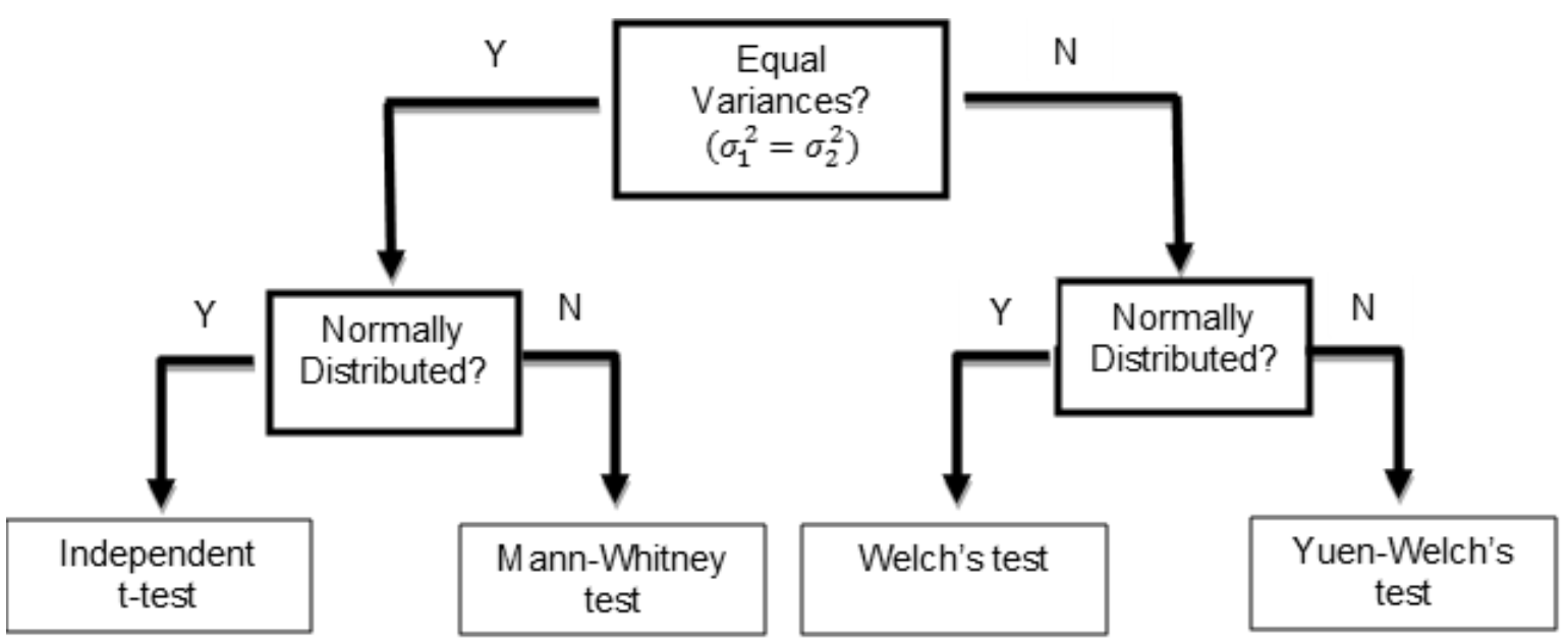
A two-sample test procedure is often presented in the form of a decision tree. Figure 1 shows a two-step test procedure when comparing two independent samples. The test procedure includes both equal variance and normality preliminary tests.

Notice in Figure 1 that the Independent t-test is the default test, because without evidence to reject the assumption of normality or equal variances, the Independent t-test is performed.

Hoekstra et al. (2012) studied whether 30 PhD students checked fictitious data for violations of the assumptions of the statistical tests they used. Hoekstra et al. found that the assumptions were rarely checked; in fact, the assumptions of normality and equal variances were formally checked only in 12 per cent and 23 per cent of cases, respectively. When the PhD students were asked the reason behind them not checking the assumptions, for the assumption of normality, approximately 90 per cent of them said it was because they were unfamiliar with the assumption; similarly, approximately 60 per cent of the PhD students gave the same reason for not checking the assumption of equal variances.

Wells and Hintze (2007) suggested that the assumptions should be considered in the planning of the study as opposed to being treated almost as an afterthought. The authors recommended considering assumptions at the planning stage: testing using prior data from the same/similar source; using theoretical knowledge or reasoning, and addressing the assumptions before the data is collected, which can avoid the issues surrounding preliminary testing. Wells and Hintze finished by suggesting that studies should be designed to be, and statistical analyses selected that are, robust to assumption violations, i.e. equal-sized groups or large sample sizes whenever possible. Equal-sized groups are desirable due to most two-sample tests that assume equal variances being robust against violations when there are equal-sized groups; for example, the Independent t-test (Nguyen et al., 2012; Derrick et al., 2016).

Zumbo and Coulombe (1997) warned of at least two scenarios where equal variances cannot be assumed: when the groups of experimental units are assembled based on important differences such as age groups, gender or education level; or when the experimental units differ by an important, maybe unmeasured variable. Thus, ideally it is the design of the experiment that should determine whether this assumption is true, not the samples collected.

At the 5% significance level, a valid test procedure should reject the null hypothesis approximately 5 per cent of the time; this would represent Type I error robustness. Rochon et al. (2012) investigated the Type I error robustness of the Independent t-test and the Mann-Whitney test. Interestingly, the unconditional test (i.e. no preliminary test) controlled Type I error rates for both two-sample tests under normality and exponentially distributed data. There may be little need for preliminary tests if the conditional tests are robust to minor deviations from the assumptions.

Garcia-Perez (2012) and Rasch et al. (2011) highlighted the ramifications of checking assumptions using the same data that is to be analysed: if the researchers do not test the assumptions, they could suffer uncontrolled Type I error rates; or they can test the assumptions but will surrender control of the Type I error rates too. 'It thus seems that a researcher must make a choice between two evils' (Garcia-Perez, 2012: 21). Any preliminary assessment of assumptions can affect the Type I error rate of the final conditional test of interest; Ruxton (2006) and Zimmerman (2004) advise against preliminary testing.

Many textbooks recommend checking the assumptions of normality and equal variances graphically; for example, Moore et al. (2018). However, Garcia-Perez (2012) emphasised that the problem of distorted Type I errors still persists because the decision on what technique to use is conditioned on the results of this graphical preliminary analysis, just like a formal hypothesis test. A graphical approach also introduces a further element of researcher subjectivity.

When preliminary testing for normality was performed, Rochon et al. (2012) have shown that the conditional Mann-Whitney test had elevated Type I error rates for the normally distributed data. Similarly, when preliminary testing, the conditional Independent t-test had large Type I error rates for the exponential distribution and uniform distribution; likely due to the lack of times it is performed, where tests for normality are performed on non-normal data. Rochon et al. concluded that for small samples, the Shapiro-Wilk test for normality lacks power to detect deviations from normality. However, this may be a good thing for a preliminary test due to the Independent t-test's robustness against violations of normality and its high power; in fact, the Kolmogorov-Smirnov test has less power than the Shapiro-Wilk test (Razali and Wah, 2011) and is often preferred. Rochon et al. also suggested that if the application of the Independent t-test is advised against due to potential concerns over normality, then the unconditional use of the Mann-Whitney test is the most appropriate choice.

Other ad-hoc methods for selecting a test to compare the central location of two samples include looking at sample size or skewness. Fagerland (2012) recommends the Mann-Whitney test for small sample sizes. Rasch et al. (2007) suggest to always perform Welch's test when there are unequal sample sizes. Penfield (1994) recommends the Mann-Whitney test when the samples are highly skewed (i.e. non-normal). However, Fagerland and Sandvik (2009) found there was no clear best test across different combinations of variance and skewness. Another ad-hoc method for selecting the most appropriate test is to assess for outliers, and perform the Mann-Whitney test or the Yuen-Welch test if an outlier is identified (Derrick et al., 2017). This highlights the amount of literature on the subject without a clear consensus.

A further complication is the choice of the 5% significance level mostly used in all preliminary tests. The 5% significance level is an arbitrary level suggested by statisticians, so it is not necessarily the optimal significance level for every application. Standard thinking regarding statistical inference at the 5% significance level is to be challenged (Wasserstein and Lazar, 2016).

In this paper, a simulation study investigates the Type I error robustness of the two-sample test procedure outlined in Figure 1. The procedure is investigated for two commonly used normality tests and two commonly used tests for equal variances, each performed at varying significance levels.

Simulation methodology

Serlin (2000) explained that in testing robustness, running simulations is the standard and appropriate approach. The simulation approach, where numerous iterations are run, generates the long-run probability of a Type I error; for each individual test, there is either a Type I error or not, and performing this process numerous times allows us to calculate the Type I error rate.

In a two independent samples design, each of the Independent t-test (IT), Welch's test (W), the Mann-Whitney test (MW) and the Yuen-Welch test (YW) are performed.

The normality preliminary tests considered are the Shapiro-Wilk test (SW) and the Kolmogorov-Smirnov test (KS). The tests for equality of variances considered are Levene's test using means (LMean) and Levene's test using medians (LMed). Each preliminary test is performed on each conditional test. The preliminary tests are performed at the 1% and 5% significance levels. The conditional test is selected based on the results of each of the preliminary tests and performed at the 5% significance level.

To account for both normally distributed data and skewed distributions, the distributions considered are Normal, Exponential and Lognormal. The Normal distribution is considered for both groups sampled from distributions with means of zero. Firstly, where both groups have variances equal to one. Secondly, groups sampled from the Normal distributions with unequal variances {1, 2, 4} are considered. Observations from the exponential distribution are generated with a mean and variance of 1. Observations from the Lognormal distribution are generated with a mean of 0 and variance of 1. Thus, in effect four separate sets of simulations are performed.

For each set of simulations, sample sizes for each of the two groups are generated in a factorial design {5,10,20,30}, i.e. 16 sample size combinations, and 10,000 iterations are performed for each combination. Emphasis is on small sample sizes, reflecting practical application.

To calculate the Type I error rates of the conditional test procedure in Figure 1, for each combination of sample size, the weighted averages of the Type I error rates for the two-sample tests performed are taken; this provides one overall value to represent the test procedure's performance. The weighting for the Type I error rates is how often the test is performed; the two-sample test performed most often is likely the most appropriate test (i.e. its assumptions match the characteristics of the two samples distributions) and should have the largest influence on the Type I error rate. Simply taking averages is not fair because one test may only be performed a small percentage of the time; similarly, reporting each conditional test Type I error rate separately is not fair because it does not consider how often the test is performed.

The Type I error rates in this study are ideally 5% because two-sample tests are designed so that their Type I error rate should match that of the significance level being tested at. These will be scrutinised in conjunction with Bradley's liberal criterion (Bradley, 1978), which says that a robust or stable Type I error rate is between 2.5% and 7.5% when testing at the 5% significance level. To determine what two-sample test or test procedure has the most robust Type I errors across the four distributions Normal (Equal variances), Normal (Unequal variances), Exponential and Lognormal distributions, it is proposed that the average absolute deviation from 5% across the four distributions is examined.

Results

Before the conditional test procedure, which uses preliminary tests, is assessed, the unconditional performance of the four tests across the four distributions must first be considered. The unconditional performance refers to the different two-sample tests Type I error rates when performed; regardless of whether the assumptions are met or not, no preliminary tests are performed. In Table 3, the 'Overall Type I Error Rate' refers to the average of the Type I error rates for the combinations of sample size and variances (when using the Normal distribution) for the two samples.

Table 3 shows that simply disregarding all assumptions and performing the Independent t-test unconditionally may not be the most robust approach. The Mann-Whitney test has the most robust Type I error rates across the four distributions since the average of the absolute deviations from 5% across the four distributions is the smallest. When looking at the test with the most Type I error control for each of the four distributions, the Independent t-test is most robust under the Normal distribution and equal variances; the Mann-Whitney test is most robust under the Normal distribution with unequal variances and the Exponential distribution; and Yuen-Welch's test is the most robust under the Lognormal distribution. It is worth noting all these Type I error rates are within Bradley's liberal criterion, so they all control the Type I error.

Figure 2 shows the distribution of the 16 Type I Error Rates for the different combinations of sample sizes (96 for the Normal Distribution under unequal variances). 'Normal EV' and 'Normal UEV', refer to the Normal distribution under equal and unequal variances respectively. The dotted horizontal lines represent Bradley's liberal criterion boundaries.

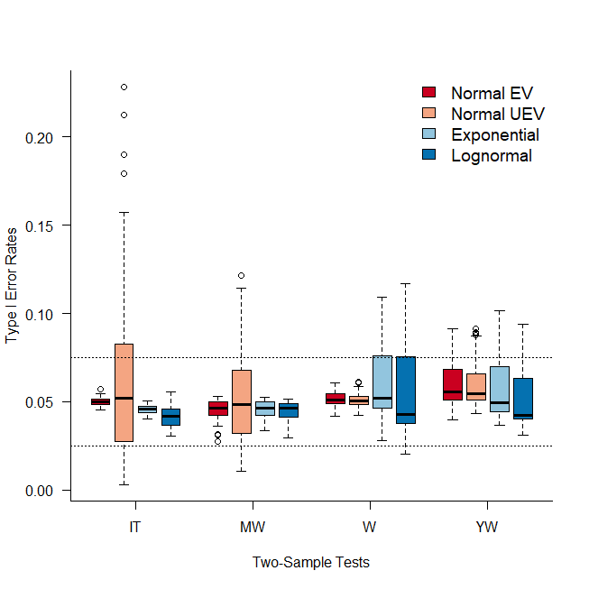
None of the two-sample tests considered control the Type I error rates for all combinations of sample size across the four distributions. The largest violations occur when there are large disparities in sample size. Therefore, performing any of the four two-sample tests unconditionally will provide Type I error rates outside of Bradley's liberal criterion for specific combinations of sample size and variances. Thus, a preliminary testing procedure may be required.

The test procedure with both normality and equal variance preliminary testing as per Figure 1 is considered. This two-stage preliminary test procedure provides 16 combinations of preliminary tests considered in a factorial design, i.e. two normality tests (SW and KS), two equal variances tests (LMean and LMed), two significance levels for the normality tests (1% and 5%) and two significance levels for the equal variances tests (1% and 5%).

The best preliminary test combinations for each distribution was assessed. For each of these preliminary test combinations, the average absolute deviation from 5% across the four distributions is given in Table 4.

For the two non-normal distributions, the Shapiro-Wilk normality test is preferred. When drawing from the non-normal distributions, normality needs to be rejected as often as possible to provide better Type I error rate control; therefore, the Shapiro-Wilk test, which does this more often, is the better normality test in this case. The average weighted Type I error rates are comfortably within Bradley's liberal criterion, with the Type I errors from the Normal distribution with unequal variances being the worst.

Table 4 shows that the two-step test procedure with Kolmogorov-Smirnov and Levene's (Mean) preliminary tests, both at the 5% significance level, achieves the most Type I error rate control. However, there is negligible difference between each of the preliminary test combinations to be of real practical consequence.

Conclusion

This paper examines some of the standard statistical tests for comparing two samples. Results show that the Independent t-test's Type I errors were less robust than the Mann-Whitney's and Welch's, but still within Bradleys liberal robustness criterion; therefore, it is not necessarily a bad choice for the default two-sample test, just not necessarily the best. Wells and Hintze (2007) and Rasch et al. (2011) also question why the Independent t-test is considered the default two-sample test and suggested using Welch's test as the default. These results further advocate a theory that the approach be revised so that Welch's test is the default.

In this paper, procedures with preliminary hypotheses tests are examined to replicate the conditions many users face when comparing two independent samples. The weighted average Type I error rates for each combination of preliminary tests were considered. Taking averages with Type I error rates does have its limitations since robust Type I error rates are defined in a range; the limitation of this is that it is possible to have equally non-robust Type I error rates either side of 5%, that when averaged, it provides a robust Type I error rate, which is not the case. However, it is more likely the test procedure has either consistently liberal or conservative Type I errors due to the changes in sample size and variances considered being relatively small, making switches from liberal to conservative Type I errors less likely. The implication of this is that, when averaged, the weighted Type I error rate will identify either a liberal or conservative Type I error rate, if the set of Type I error rates are truly liberal or conservative, instead of showing robust Type I errors when the set of Type I errors is not.

When comparing the two-sample tests performed unconditionally to the conditional testing procedure, the weighted Type I errors across the four distributions for the recommended conditional test procedures were comparable and more robust in most cases. This implies that despite the test procedures introducing compounded errors caused by the preliminary tests, the weighted Type I error rates were better for it, because the most appropriate test was performed more often.

For the scenarios considered, the benefits of implementing a test procedure to find the most appropriate two-sample test may outweigh that of performing a two-sample test unconditionally in terms of controlled Type I error rates across the four distributions. However, it is advised if possible to follow Wells and Hintze's (2007) advice of determining whether the sample size is large enough to invoke the Central Limit Theorem; considering the assumptions in the planning of the study; and testing assumptions if necessary from a similar previous data source.

The preliminary testing procedure that most closely maintains the Type I error rate is preforming Kolmogorov-Smirnov normality test and Levene's (Mean) test for equal variances, both at the 5% significance level. The test procedure performs well, with robust Type I errors when data considered is from either the Normal distribution or the skewed distributions. However, the use of a flow diagram and this rule to select the 'appropriate' test can encourage inertia and restrict critical thinking from the user about the test being performed.

Given the capacity for different researchers to conduct potentially conflicting analyses, solutions that offer the most transparency and forward planning are recommended. This is leading to some disciplines requesting that analysis plans are pre-registered, examples include the Journal of Development Economics and the Center for Open Science. This would seem like an appropriate way forward.

Acknowledgements

I would like to thank my Mum and Dad first and foremost for their support throughout my degree. I would also like to show my appreciation towards my A-Level Maths teacher Mr Gray, who did more for me in six months than any other teacher; as well as Mrs Doran who helped me throughout the whole seven years at school. Acknowledgement is given to three anonymous reviewers for their thorough discussion based on this paper. Thanks also goes to Dr Paul White for his invaluable advice on this paper and all things stats……. Jack

To cite this paper please use the following details: Pearce, J & Derrick, B. (2019), 'Preliminary Testing: The devil of statistics?', Reinvention: an International Journal of Undergraduate Research, Volume 12, Issue 2, https://reinventionjournal.org/article/view/339. Date accessed [insert date]. If you cite this article or use it in any teaching or other related activities please let us know by e-mailing us at Reinventionjournal@warwick.ac.uk.