Joseph Thomas Brooks, University of Warwick
Throughout the COVID-19 pandemic, the use of non-pharmaceutical interventions (NPIs), including lockdown measures, by governments around the world has been informed by mathematical modelling. Broadly, these models look to gauge how well NPIs control disease transmission. Here we present a model that not only forecasts the effectiveness of NPIs in restricting contacts but also assesses their influence on the mental wellbeing of affected populations. Our model is informed by data from the United Kingdom Time Use Survey, 2014-2015. This survey recorded the time participants spent in different social settings as well as self-reported enjoyment in these settings, allowing us to augment a quantitative model of social contact behaviour with associated wellbeing estimates. We use this model to assess the effectiveness of NPIs aimed at reducing social contacts in different settings and estimate their impact on population-level wellbeing. Our findings indicate that workplace closures represent the most effective intervention for slowing disease spread, while NPIs targeting other contact locations have comparatively limited impacts on transmission. Our model suggests that workplace closures not only effectively reduce infections but also have a relatively modest effect on population wellbeing levels.
Keywords: Mathematical epidemiology, infectious diseases, COVID-19, wellbeing modelling, mixing patterns, time-use surveys.
Since early 2020, governments have worked to control the COVID-19 pandemic. Prior to the development of vaccines, non-pharmaceutical interventions (NPIs) were the primary method of reducing infection for governments (Hale et al., 2021). In the years following the outbreak of the pandemic, there has been a rapid expansion in the literature assessing various NPIs, including mask wearing, school closures, lateral flow testing and travel restrictions in populations around the world (Banks et al., 2020; Dimeglio et al., 2021; Flaxman et al., 2020; Jarvis et al., 2020; Lai et al., 2020; Leng et al., 2022; Perra, 2021; Firth et al., 2020; Prem et al., 2020; Silva et al., 2021). However, when assessing the success of these measures, it may be necessary to consider the potentially damaging effects that measures such as school and work closures have on the mental and emotional wellbeing of the affected population (White and Van Der Boor, 2020).
Early reports of COVID-19 indicated a strong age-stratified component in epidemiological risk, a suggestion that has been validated over the course of the pandemic (Li et al., 2020; O’Driscoll et al., 2021). Building on previous developments in infectious disease modelling (Anderson et al., 1986; Keeling and Rohani, 2007; Schenzle, 1984), age-structured infectious disease models were widely used to model the dynamics of the COVID-19 pandemic (Davies et al., 2020; Hilton et al., 2022; Hilton and Keeling, 2020; Moore et al., 2021; Prem et al., 2020).
The transmission of respiratory infections such as COVID-19 is driven primarily by social contacts, making it important that relative intensities of the age-stratified transmission pathways in these models reflect high-quality real-world estimates of age-stratified contact rates. The ‘contact survey’ methodology developed in the widely influential POLYMOD study (Mossong et al., 2008), and which has since been expanded upon in other large studies such as Prem et al. (2021), can be used to calculate contact matrices which quantify mixing patterns in a stratified population. An alternative source for age-stratified contact rate estimates is time-use surveys. These surveys collect data on how individuals spend their time (i.e. location, activities) from which researchers can infer empirical estimates of the mixing patterns of a population. Time-use surveys have previously been used to determine mixing patterns for epidemiological modelling in Zagheni et al. (2008), who developed a methodology to estimate time-of-exposure matrices summarising the risk of infection over time in different social settings. Dynamic models of infectious disease have also been developed using data from POLYMOD (Fumanelli et al., 2012), time-use data (Ajelli et al., 2014) or a combination of the two (van Leeuwen et al., 2022) to inform their mixing patterns. The latter (van Leeuwen et al., 2022) employed time-use data to augment contact matrices to reduce contacts by activity, thereby enabling the simulation of fine-grained interventions.
In this study, we build on previous studies of age-structured infectious disease dynamics by augmenting an age-stratified contact model with an estimate of how changes in social contact behaviour induced by NPIs can impact societal wellbeing. Our model works by estimating the basic reproductive ratio, a fundamental epidemiological quantity determined by both the biology of the pathogen in question and the social dynamics of its host population, from age-stratified estimates of a population’s time-use behaviour. These time-use estimates summarise the time spent exposed to different sections of the population, from which we can estimate the basic reproductive ratio, but also the population’s self-reported enjoyment associated with different social settings, which we use as a proxy for population-level wellbeing. We model the impact of NPIs by manipulating the age-stratified time-use profile to reflect the impact of changes to social contact behaviour (for instance, by reducing average time spent in work settings and increasing time spent in home settings by a corresponding amount), and then calculating the resulting values of basic reproductive ratio and population-level wellbeing under this modified time-use profile. This allows us to identify combinations of measures that are likely to reduce transmission of infection while minimising harmful impact on population-level wellbeing.
We used data from the UK Time Use Survey 2014-2015 (TUS) (Gershuny and Sullivan, 2017) to generate age-structured contact matrices quantifying the expected amount of social contact between age groups. The TUS covered over 10,000 participants and recorded their location and activities at a 10-minute temporal resolution, providing a highly granular sample of population behaviour. Further details on the TUS and how it was used in this investigation can be found in Appendix A. The age-structured contact matrices we derive are analogous to the social contact matrices estimated in studies such as the POLYMOD study of Mossong et al. (2008) and Prem et al. (2021). Whereas estimates from social contact surveys will only account for contacts that individuals have remembered and recorded, estimates from time-use surveys have the potential to capture more diffuse casual contacts. Following the methodology of Zagheni et al. (2008), the social contact intensities we generate are to be interpreted as the relative risk to an individual of age class from the aggregate of individuals of age class in a given location on a single day. This exposure level is measured in person-hours: 1 hour spent in contact with 1 person; if an individual of age class has probability of being in location in hour and there are an expected individuals of age class in that location in hour , then the expected number of person-hours is . The resulting contact matrices are not symmetric because the probability of encountering an individual in a given age class is dependent on, among other factors, the proportion of the population that are in that age class. For example, there are many more individuals in the UK aged 25-29 than aged 80-84 (ONS, 2024). This means that a single individual aged 80-84 will make many more contacts with 80–84-year-olds than in the other direction. We generate matrices for each location listed in the UK TUS and aggregate them into three broad location categories: ‘external’ interactions, capturing all non-home locations; ‘within-household’ contacts, capturing contacts between members of the same household; and ‘other home’ contacts, corresponding to an individual’s interactions in a household setting which is not their own home. This aggregation is made to reflect the fact that mixing behaviour in each of these three categories is extremely different and is treated separately; contact within a household are likely to be much more intense than those in an external location such as a workplace. A summary table of the locations recorded by the survey, including the categories into which we placed them, can be found in Appendix C.
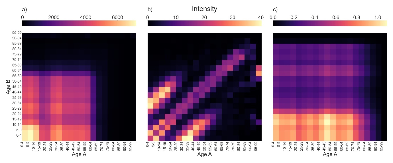
In Figure 1, we visualise the location-specific contact matrices generated from the TUS data. Details on the construction of these matrices can be found in Appendix B. Our contact intensity calculations assume that external contacts involve exposure to the general population, whereas within-household contacts are limited to those individuals present in a single household, and so the ‘external contacts’ intensities are of a higher order of magnitude than both sets of household-based contact intensities. External contacts (Figure 1a) are characterised by intensive mixing of younger age groups, likely at school, and a sharp decrease past age 65. Within-household contacts (Figure 1b) show a highly age dependent structure, with strong mixing of people of the same age as well as contacts between carers and children being clearly visible in the two smaller branches either side. Other home mixing (Figure 1c) is characterised by frequent contact between young individuals and individuals of all ages, indicating that younger people are more likely to be visiting individuals in another home than individuals aged 20+. These qualitative patterns are consistent with those found in previous studies of time-use data (Zagheni et al. 2008), and the distinctive three-armed shape of the within-household mixing matrix is similar to that seen in the POLYMOD study (Mossong et al., 2008).
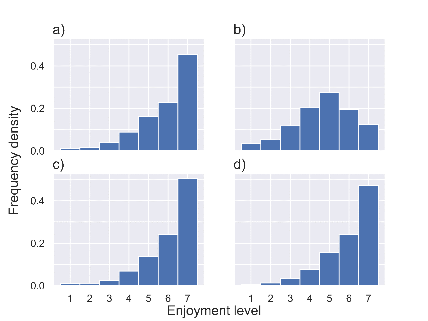
We analyse the epidemiological impact of NPIs by estimating the effective reproductive ratio which results from a specific package of NPIs. The basic reproductive ratio, , is defined as the average number of people infected by an infected person at the early stages of an outbreak, while the effective reproductive ratio, , is defined analogously as the average number of people infected by an infected person under a given set of control measures. These reproductive ratios can be obtained through eigenvalue calculations on social contact matrices (Keeling and Rohani, 2007), such as the ones we obtained from TUS data. We first assume a value of and scale the contact matrix appropriately so that it reflects this value. We can thus estimate the impact of NPIs by adjusting the contact matrices to reflect behavioural changes and then calculating the resulting effective reproductive ratio, as detailed in our Appendices D and E. Throughout these calculations we assume a constant rate of recovery – assumed to be 1/7 so that the expected length of infection is seven days. We augmented this projection of epidemiological impact by estimating the impact of NPIs on population wellbeing using the estimates of reported enjoyment by location provided in the TUS data. We make wellbeing calculations first under the ‘best-case scenario’ assumption that additional time spent at home takes the same enjoyment value as time otherwise spent at home. Additionally, we consider a ‘worst-case scenario’ in which all additional time spent at home is assumed to take the lowest enjoyment value of 1. See Appendix F for further details on enjoyment calculations and Appendix G for distributions of enjoyment levels in selected locations.
We analysed the effect of three basic classes of NPI on and wellbeing levels. These NPIs were closure of workplaces and schools, a prohibition of visits to other households, and the closure of leisure locations such as hospitality establishments, sports centres, art museums and shops. For each of these measures, we calculated reproductive ratios and projected enjoyment scores as a function of the degree of stringency of the measure, defined to be the proportion of total time spent in a location which is replaced by time at home under the NPI. An NPI with stringency affecting location should thus be interpreted as scaling the probability that an individual is in location at a given time by , with the resulting ‘lost’ time being balanced by an increase in the probability that they are at home at that time. An NPI of stringency would thus require all individuals to stay home whenever they would usually be at the location affected by the NPI, while an NPI with stringency would have no impact on time use. Calculations around the implementations of NPIs are covered in Appendix D. To account for uncertainty in the relative contributions to the population-level epidemic made by within- and between-household transmission, we repeat our analysis for three different values of the susceptible-infectious transmission probability (SITP) (House et al., 2022). This quantity, which we denote , is defined as the probability that a susceptible individual is infected by the index case of an outbreak in their household. For each value of the SITP, we assume a baseline pre-NPI reproductive ratio of , which is largely consistent with the range of estimates for the reproductive ratio of wild-type COVID-19 produced in 2020 (Liu et al., 2020). Our analysis thus focuses on COVID-19-like population-level spread but explores uncertainty in the relative contributions to this spread of within- and between-household transmission, with models with lower SITPs having higher levels of between-household spread to compensate. The effect of the value of on the contributions to the value of of different locations can be seen clearly in Table 1.
| p = 0.25 | p = 0.5 | p = 0.75 | |
| Within-household | 8.83% | 17.66% | 26.49% |
| Other home | 0.78% | 1.86% | 3.67% |
| Work | 85.02% | 75.69% | 65.69% |
| Leisure | 2.11% | 1.88% | 1.63% |
In Figure 2, we plot the estimated effective reproductive ratio and the projected mean enjoyment score as a function of the stringency of NPIs affecting schools and workplaces (Figures 2 a)–c)), visits to other households (Figures 2 d)–f)) and locations associated with leisure activities (Figures 2 g)–i)) under the assumption of weak (), intermediate () and strong within-household transmission (). Our results suggest that school and workplace closures are by far the most effective measure, although achieving an effective reproductive ratio below the critical epidemic threshold of is only possible with highly stringent measures and when levels of within-household transmission are low. This reflects the much higher proportion of time spent at work (10.5 per cent) than in other people’s homes (3.2 per cent) and in locations associated with leisure (4.7 per cent) in the TUS. Additionally, the commonality of a shared work/school day among the working and school-aged population further amplifies the absolute impact of proportional changes in time use, particularly accentuating the significance for work locations compared to other settings.
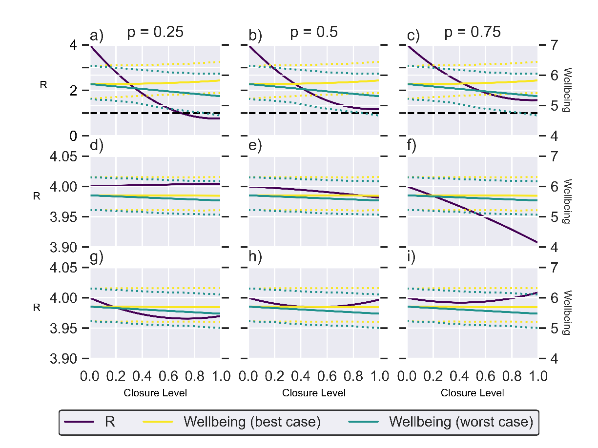
In general, the effectiveness of an NPI decreases with an increased level of within-household transmission because some of the external infections that are prevented by the NPIs are offset by an increased potential for infection within the household. The non-linear shape of the curves in Figure 2 demonstrate this offset, with highly stringent measures offering diminishing returns. This is particularly pronounced for closures to leisure (Figures 2g)–i)). Since people spend relatively little time in leisure locations – and that time is less likely to overlap with others than say time spent at work – there is lower risk of infection in those locations. Therefore, stringent measures that result in a lot of that time being spent at home, a higher risk location, may result in a higher reproduction ratio than the base scenario with no NPIs.
Under the best-case scenario model, the NPIs have negligible to positive effect on wellbeing levels since individuals in the TUS generally reported higher enjoyment when at home than at work, and similar levels of enjoyment for time spent at home and on leisure activities away from home. Therefore, when NPIs are implemented and time spent at work or in leisure locations is moved to time spent at home, the wellbeing measure increases or is unchanged respectively. At the opposite extreme, the worst-case scenario model predicts a significant negative effect on population-level wellbeing. As is the case for the effective reproductive ratio, we see much more substantial changes in wellbeing under school and workplace closures than under the other NPIs as a result of the large amount of time spent in the workplace. The inter-quartile range (IQR) for the wellbeing under each wellbeing scenario are shown by the dotted lines. This is the IQR for all wellbeing scores, not a projection of the IQR under no intervention.
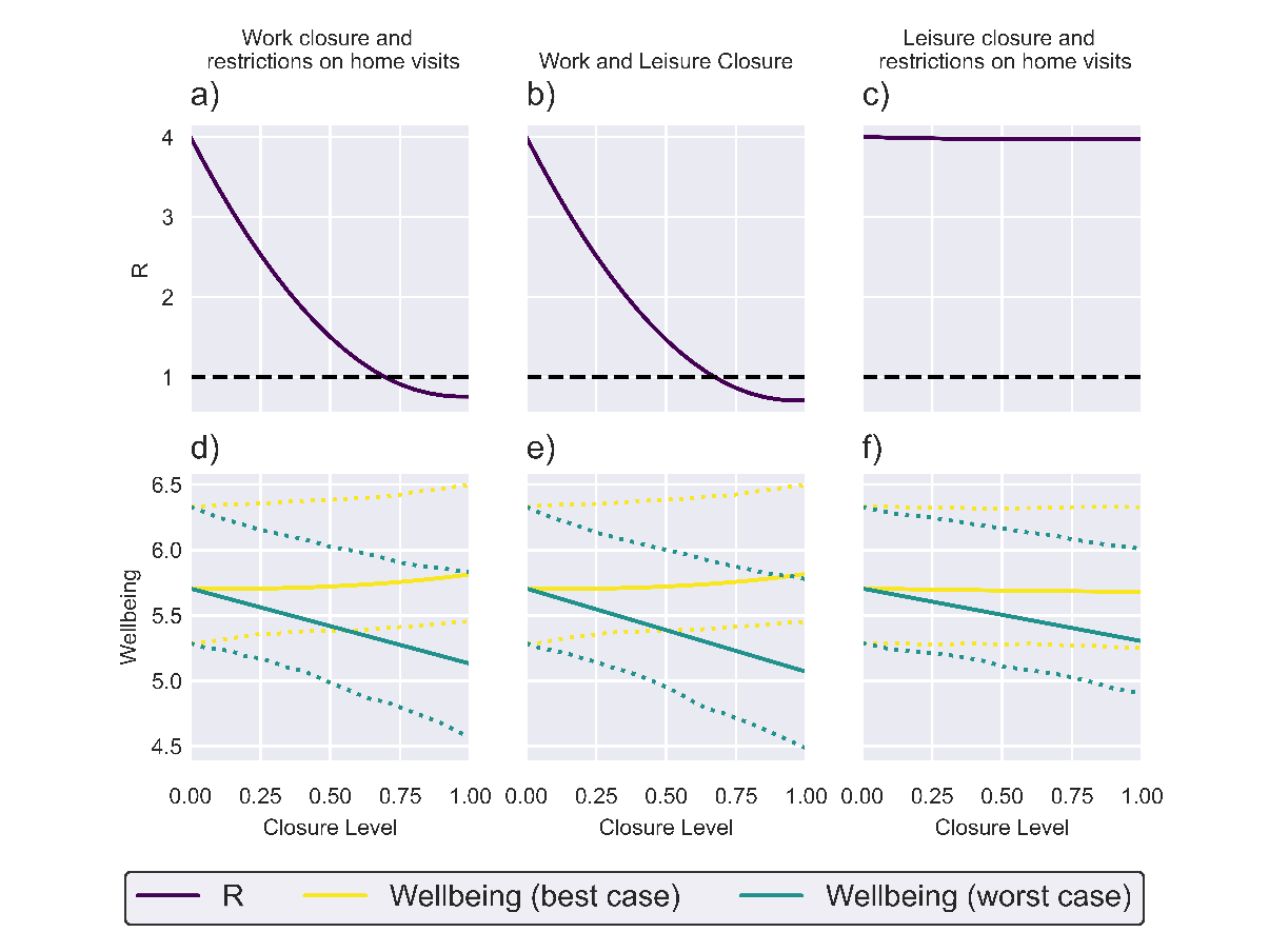
The projected impacts of implementing packages of NPIs targeting two categories of transmission environment are plotted in Figure 3. Packages including work closure measures (Figures 3a), b), d) and e)) are projected to be capable of bringing the effective reproductive ratio below 1, consistent with the single-route analysis which projected that work closures would be substantially more effective than restrictions targeting other routes of transmission. Our simple wellbeing model suggests that under best-case scenario conditions, these packages will have minimal impact on mean enjoyment levels, while causing a more substantial reduction in mean enjoyment than work closures alone under worst-case scenario conditions. Targeting public leisure activities and visits to other homes (Figures 3c) and f)) is projected to have minimal impact on the effective reproductive ratio while having minimal impact on mean enjoyment under the best-case scenario and substantially reducing mean enjoyment under the worst-case scenario.
In this study, we have used a simple mathematical model to assess the impact of NPIs both in an epidemiological sense and in terms of their potential impact on population-level wellbeing. The large sample size and fine temporal resolution of the TUS data allowed for detailed modelling of the behavioural impact of different NPI packages. Our results suggest that reductions in time spent at work are likely to have a much higher impact on the spread of infection than restrictions targeting leisure activity and household visits while having minimal impacts on population-level wellbeing. This reflects the long durations spent at work recorded by many TUS participants and the comparatively low levels of enjoyment recorded there. There is thus a substantial accumulation of person-hours in these locations, concentrating the risk of disease exposure in this location. In scenarios where transmission is primarily along external rather than within-household lines (i.e. the SITP is small), work closures are sufficient to bring below 1. In contrast, the combination of relatively short durations and high enjoyment levels recorded by TUS participants in leisure locations and at other households means that interventions focusing on these locations are projected to have minimal impacts on infectious disease transmission and negative impacts on population-level wellbeing.
Our epidemiological findings – namely that work and school are the location that contributes the most to the reproductive ratio and restrictions to these locations have the largest impact on infection spread – agree qualitatively with results of van Leeuwen et al. (2022). Davies et al. (2020) find that NPIs alone are unlikely to be sufficient to reduce the reproductive number below 1, and thus control an outbreak, unless full ‘lockdown’ measures are taken. Van Leeuwen et al. (2022) also finds that limiting contacts in only one category of location – for example, other home visits or shops – is not enough to reduce case numbers significantly. This agrees with our findings that the selective closure of environments is insufficient and high levels of closure of workplaces and schools would be necessary to achieve a reproductive ratio below 1.
The wellbeing model we have proposed here represents a simple ‘first order’ approximation of actual psychological responses to NPIs, intended to point the way forward to more detailed and realistic combinations of epidemiological and psychological dynamics. In practice, the like-for-like approach we have taken to our enjoyment calculations, with each block of time taking an independently assigned enjoyment value based on location, is unlikely to reflect actual human psychology. Our model could be expanded upon to take a more holistic approach to reflect overall wellbeing – for instance, by reducing enjoyment levels in proportion to the degree of disruption caused by NPIs. At the finer scale, using recorded activities alongside location to determine projected enjoyment levels could offer an improvement. In particular, our projected increase in mean enjoyment resulting from workplace restrictions may reflect enjoyment levels recorded at home mostly corresponding to leisure time, and it is possible that we will see different responses if we replace enjoyment levels recorded in the workplace specifically with levels recorded for time spent working at home in the TUS.
The main strength of our epidemiological model is its coupling to a model of wellbeing, with our basic approach pointing the way towards more complex models with the potential for much greater public health impact. In this study, we have carried out reproductive ratio calculations rather than generating medium- to long-term projections of the infectious disease dynamics. Dynamic models with social contact structures derived from the UK Time Use Survey 2014-2015 have been used to project the impact of NPIs (van Leeuwen et al., 2022) and are a natural candidate for augmentation with a wellbeing model based on the TUS data. Our calculations focused heavily on the distinction between within- and between-household transmission and could be extended into a fully dynamic household-stratified transmission model based on previous stochastic and deterministic models of infection at the household level (House and Keeling, 2009; Hilton et al., 2022; Ross et al., 2010).
Future iterations of our model could offer improvements in realism by incorporating a more explicit social network structure; one of the reasons for the vast difference in person-hours of exposure at the household-and-workplace level is that we modelled households as a small finite unit of population, whereas all individuals recorded as being ‘at work’ during a given time slot in the TUS were assumed to have some degree of exposure to one another. In practice, workplaces are highly segregated, with individuals at work typically being exposed mainly to individuals who share their workplace (although individuals in retail or service jobs are an important exception to this principle). A potential solution to this would be to refine the model by incorporating statistics on the size of workplaces so that an upper limit could be placed on person-hours of exposure in the workplace. Alternative aggregation of locations into more categories could also be made to reflect different patterns of mixing and behaviour. For example, one might expect that workplace contacts would be more intense than those in other ‘external’ locations. However, this would involve adding an extra parameter to the model to distinguish between the per-unit-time transmission rates for work and non-work locations. In this study, we have retained a two-parameter formulation that in a real-world setting would allow the model to be parameterised from population-level incidence data and within-household epidemiological studies, both of which were available during the COVID-19 pandemic. Similarly, the ‘leisure’ location in our model represents an aggregate of many non-overlapping contact sites. Social contacts in the workplace also tend to be repetitive, with individuals seeing the same set of people at work every day. In a dynamic model, this means that as immunity builds up in a workplace through repeated infection, the workplace will become a less risky site of social contact with respect to infection, and this build-up of local immunity is not accounted for in our approximation of the workplace as a single fully connected population unit. The weaknesses stemming from our unrealistic assumptions around workplace and leisure contacts could be remedied either by incorporating our wellbeing calculations into a model with an explicit household-and-workplace structure (Pellis et al., 2011) or through the use of a network model (Keeling and Eames, 2005). Network models have been applied both in the study of COVID-19 pandemic-era NPIs (Chang et al., 2021; Karaivanov, 2020) and in the context of wellbeing modelling to study the spread of mood within social cliques (Eyre et al., 2017).
Prior to the outbreak of the COVID-19 pandemic, research had suggested that quarantine is linked to adverse psychological outcomes (Brooks et al., 2020). Since the outbreak of the COVID-19 pandemic, numerous studies have been conducted to scrutinise the patterns in mental health before, during and after the introduction of lockdown measures. Longitudinal analyses of UK household data revealed significant increases in psychological distress, particularly among young individuals and women, after one month of lockdown, exacerbating pre-existing disparities in mental health (Banks and Xu, 2020; Chandola et al., 2022; Niedzwiedz et al., 2021). Studies found that risk factors for worse mental health included being female, having a lower income and having pre-existing mental health conditions. Among females, there was found to be much more variation in mental health compared to males, who experienced a relatively stable trajectory between April and November 2020 (Stroud and Gutman, 2021). Additionally, studies suggested that despite initial ‘shock’ factors leading to significant increases in mental disorders, anxiety and depression, levels of both declined in the first 20 weeks following the introduction of lockdown measures in England (Fancourt et al., 2020). Studies conducted to specifically look at the mental health of UK university students found that during the COVID-19 pandemic there was a significantly elevated prevalence of depressive symptoms (Evans et al., 2021; Owens et al., 2022). Owens et al. in particular found that this heightened prevalence (55 per cent of students), linked to lack of sleep, did not decrease significantly over time (52 per cent of students). These findings could inform future efforts to construct a more sophisticated model of population wellbeing, incorporating the evolution of various wellbeing metrics during an intervention and acknowledging the demographic heterogeneity highlighted by the body of research.
Dr Joe Hilton, Postdoctoral Researcher, University of Liverpool: For supervising the original project and going above and beyond in supporting the writing of this paper.
Figure 1: Estimated contact matrices for the following contact settings.
Figure 2: Single location NPI plots.
Figure 3: Two location NPI plots.
Table 1: Contributions of different locations to R0 under varying assumptions of within-household transmission probability.
Table 2: A compilation of potential location values in a specified TUS entry, accompanied by the associated infection pathway, related restrictions influencing social interactions within the location, and the percentage of time allocated (considering day-of-the-week scaling).
The model was informed by data from the UK Time Use Survey (TUS) 2014-15 (Gershuny and Sullivan, 2017). Participants in the survey filled out a diary in which they recorded their location and current activity at 10-minute intervals over the course of one weekday and one weekend day, along with a record of who they were currently with, and the level of enjoyment associated with each interval scored on a scale of 1 to 7. The diary was linked to demographic information on the participant, in particular their age. Each 10-minute interval was encoded with one of 38 different location values, which are shown in Appendix C.
Individuals were put into 20 age groups, each one a five-year interval going from 0–4 years old up to 95–99 years old. The survey only recorded diary entries for individuals who were 8 years or older, however; children aged 7 and under were included in the data on household composition. In order to still incorporate contacts involving children aged 8 or under, the assumption was made that the behaviour of children aged 0–7 could be approximated by those aged 8–9. This will not be wholly realistic, particularly for children who are not yet school age, but any discrepancies are unlikely to be significant.
We construct our pre-NPI contact matrices from time-use survey data using the method introduced by Zagheni et al. (2008). For each location option in the TUS, we calculated a contact matrix where was the approximate number of contacts a person in age group has with people in age group at the location in a day.
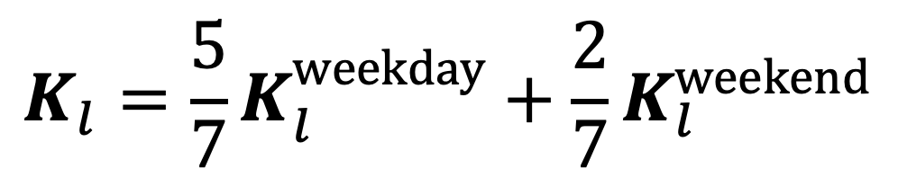
We take into account day-of-the-week effects by constructing separate contact matrices for each location based on contacts recorded on weekdays and on weekends, and then taking the weighted average of the two. Hence, the contact matrix for location , , is calculated by the weighted sum of the two:
|
Equation 1. |
|
This weighted sum is suppressed in the definitions of the various location contact matrices for ease of exposition.
We use to denote the set of 10-minute time intervals used in the TUS, so that corresponds to the 10 minutes starting at 12:00 a.m. and ending at 12:10 a.m. We use to denote the estimated probability that under the conditions of the TUS (i.e. in the absence of NPIs) during a time interval a given individual experiences a contact event of 10 minutes of exposure to a single individual of age class in a given location, .
Our model of the transmission process distinguishes between transmission within a household, between visitors and residents of a household, and at external non-household locations. In order to simplify notation, the locations coded in the TUS data as ‘Other people’s home’ and ‘Home’ will be denoted and respectively.
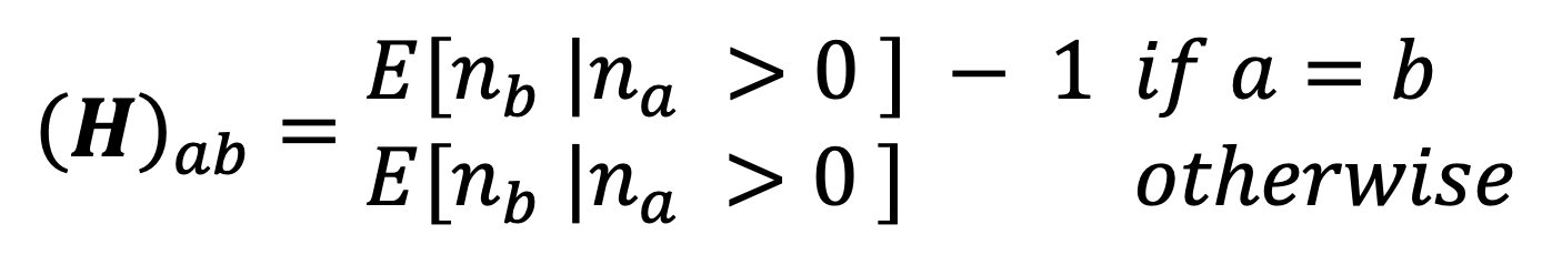
Using the household composition data from the TUS, we construct a matrix where each entry is the estimated expected number of people in age group in a household that has at least one individual in age group ,
|
Equation 2. |
|
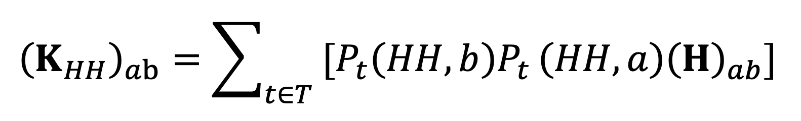
where is the number of people in age group in a given household. In the case where , 1 is subtracted to avoid counting contacts with yourself. Using this matrix, we can construct a contact matrix for mixing within the household:
|
Equation 3. |
|
Each term in the summation gives the expected number of contacts with age class members of their own household experienced by an individual of age class during a single 10-minute interval, so that gives the expected number of contacts of this type over an entire day.
We consider visits to other households as a distinct category of mixing on the basis that these contacts are likely to be with close friends and family members, meaning that they will differ from work/leisure contacts in terms of physical proximity and frequency of touch. This is reflected in the package of NPIs implemented in the UK during the height of the COVID-19 pandemic, which placed separate restrictions on household visits and work/leisure activities.
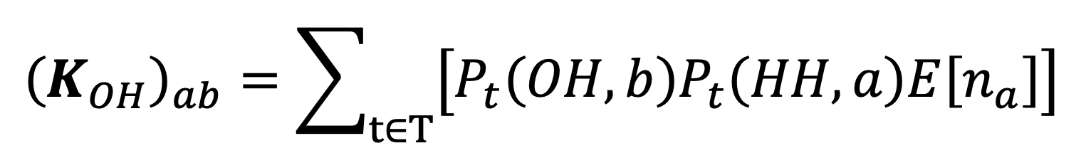
We calculate the expected number of ‘Other people’s home’-coded contacts with individuals of age class experienced by an individual of age class a follows:
|
Equation 4. |
|
Here is the average number of individuals of age class per household. Each term in the summation encodes the probability that an individual of age class spends time interval in a household other than their own, multiplied by the expected number of individuals of age class belonging to that household who are at home during that time interval. While this captures the exposure experienced by individuals visiting a household to members of that household, our model will not capture the effect of cross-contact between separate visitors to a household. Given the relatively small amount of time individuals spend visiting other households in the TUS, the effect of ignoring these cross-contacts is likely to be minor. In particular, cross-contact between members of the same household visiting a second household is very unlikely to make a substantial contribution to population-level infection since infections between members of a shared household are overwhelmingly likely to take place within their own household given the long time periods spent there.
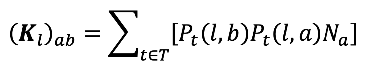
We define external contacts to be all contacts made in settings other than ‘Home’ or ‘Other people’s home’. We will denote the full set of external locations by . The expected number of contacts with individuals of age class made by an individual of age class in location during a single day is given by:
|
Equation 5. |
|
where is the total number of people in age group in the whole population. This defines a location -specific contact matrix , and summing these over all the external locations in the TUS data gives the external contact matrix we use in our analysis:
|
Equation 6. |
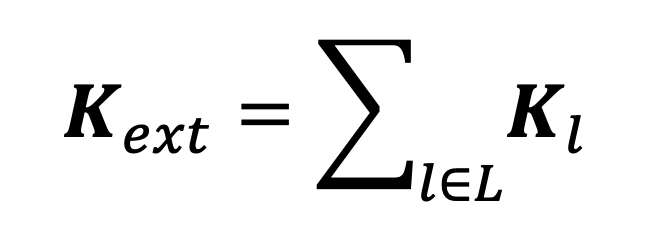
|
| Location Label | Pathway | Restrictions | Time spent (%) |
| Unspecified location | ext | 0.5753% | |
| Unspecified location (not travelling) | ext | 0.8544% | |
| Home | HH | 69.0225% | |
| Second home or weekend house | HH | 0.1956% | |
| Working place or school | ext | Work Closure | 10.5454% |
| Other people’s home | OH | Restrictions on home visits | 3.2442% |
| Restaurant cafe or pub | ext | Leisure Closure | 1.1801% |
| Sports facility | ext | Leisure Closure | 0.6378% |
| Arts or cultural centre | ext | Leisure Closure | 0.0618% |
| Parks/countryside/coast | ext | Leisure Closure | 0.4751% |
| Shopping centres markets other shops | ext | Leisure Closure | 1.3722% |
| Hotel guesthouse camping site | ext | Leisure Closure | 0.9423% |
| Other specified location (not travelling) | ext | 2.1841% | |
| Unspecified private transport mode | ext | 0.0406% | |
| Travelling on foot | ext | 1.6769% | |
| Travelling by bicycle | ext | 0.1160% | |
| Travelling by moped/motorcycle | ext | 0.0199% | |
| Travelling by car as the driver | ext | 1.8169% | |
| Travelling by car as a passenger | ext | 0.4595% | |
| Travelling by car – unspecified | ext | 1.0611% | |
| Travelling by lorry or tractor | ext | 0.1252% | |
| Travelling by van | ext | 0.2251% | |
| Other specified private travelling mode | ext | 0.0259% | |
| Unspecified public transport mode | ext | 0.0030% | |
| Travelling by taxi | ext | 0.1087% | |
| Travelling by bus | ext | 0.3901% | |
| Travelling by tram or underground | ext | 0.0760% | |
| Travelling by train | ext | 0.2260% | |
| Travelling by aeroplane | ext | 0.0423% | |
| Travelling by boat or ship | ext | 0.1096% | |
| Travelling by coach | ext | 0.0272% | |
| Waiting for public transport | ext | 0.0492% | |
| Other specified public transport mode | ext | 0.0199% | |
| Unspecified transport mode | ext | 0.7103% | |
| Illegible location or transport mode | N/A | 0.0014% | |
| No answer/refused | N/A | 1.3782% | |
| Interview not achieved | N/A | 0.0% |
In our model, NPIs act to reduce the probability that an individual is in a specific location or group of locations in a given time interval and increase the probability that they are at home in that time interval by a corresponding amount; since the total amount of time in a day is constant, any reduction in time spent in an external location must be balanced by an increase in time spent at home. We encode a specific NPI as a set of age-stratified vectors where is the probability that an individual of age class is in location during time interval relative to the equivalent probability in the absence of NPIs. The relative reduction in probability is thus given by . In this study, we will not consider measures such as curfews which only affect mixing during certain times of day, so that does not change with and we can thus suppress the time dependence and write . We will denote the set of locations affected by the NPI as >.
Under the NPI specified by , the resulting within-household contact intensities are given by
|
Equation 7. |

|
which cannot be easily expressed in matrix terms. For the home-visit contact matrix, the new contact intensities will be given by:
|
Equation 8. |

|
which also cannot be easily expressed in matrix terms. The resulting matrices for an external location, , effected by the NPI, is given by
|
Equation 9. |
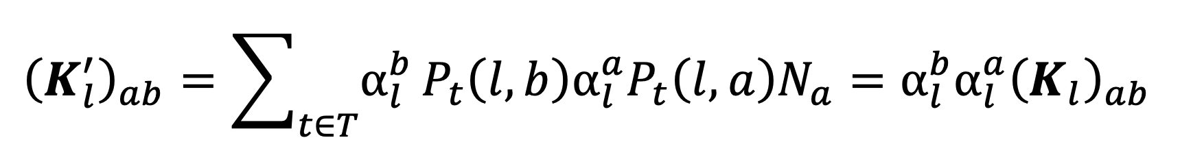
|
namely, . The external contact matrix resulting from the NPI is then given by replacing the matrices encoding locations affected by the NPI with their adjusted versions in Equation 6:
|
Equation 10. |
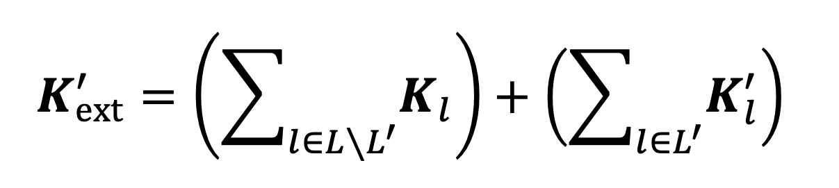
|
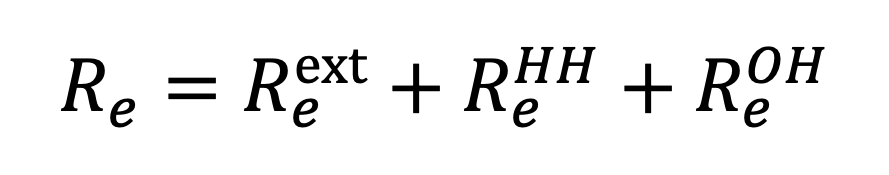
In this study we quantify the effectiveness of NPIs by estimating the effective reproductive ratio, , of the infection under a specified package of NPIs. This is defined as the expected number of secondary cases generated by a single case under conditions of low background immunity; our analysis is thus focused on the effectiveness of NPIs in terms of their ability to prevent a new pathogen from establishing itself in the population, rather than in terms of real-time application during an evolving epidemic. We distinguish the effective reproductive ratio under a package of NPIs from the basic reproductive ratio, , which is defined to be the reproductive ratio in the absence of NPIs. In what follows, we outline the calculation of the basic reproductive ratio using estimates of contact intensities derived from TUS data; the same set of formulae define the effective reproductive ratio under a package of NPIs when the underlying contact behaviours are replaced by projected contact behaviours under those NPIs.
Our model distinguishes three transmission pathways: within-household transmission (HH), defined as transmission occurring with a household between two individuals who live in that household; other household transmission (OH), defined as transmission occurring with a household between one individual who lives in that household and one who does not; and external transmission (ext), defined as transmission at any location other than within the home. Each transmission route has an associated basic reproductive ratio, defined to be the expected number of secondary infections generated along that route by a single case over the course of their infectious period in the absence of immunity, denoted within-household transmission, for other household transmission, and for external transmission. The basic reproductive ratio is given by summing these route-specific reproductive ratios:
|
Equation 11. |
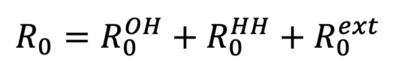
|
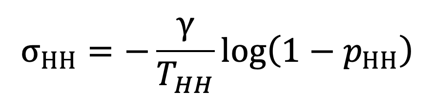
The within-household basic reproductive ratio is defined in terms of the susceptible-infectious transmission probability, the probability that a susceptible individual is infected by a single infectious individual within their own household, which we will denote . If an infectious individual transmits to each susceptible individual within their household at rate whenever both individuals are in the household, then infection events can be modelled as a Poisson process with intensity . The expected duration of this process is given by the expected time per day which both individuals are at home, , multiplied by the expected duration of infection, . The mean of the Poisson process is thus given by
|
Equation 12. |
|
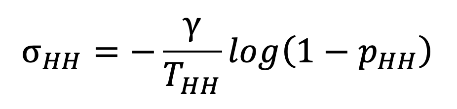
The susceptible individual is infected the first time an event occurs in the Poisson process, so that the probability that they are not infected during the infectious individual’s infectious period is given by , where . The SITP is thus given by
|
Equation 13. |

|
In practice, the SITP can be estimated empirically from longitudinal studies of infection (House et al., 2022), while the pairwise transmission rate cannot be measured directly. Given an estimated infectious period and an average contact duration estimated from the TUS, we can rearrange Equation 13 to get
|
Equation 14. |
|
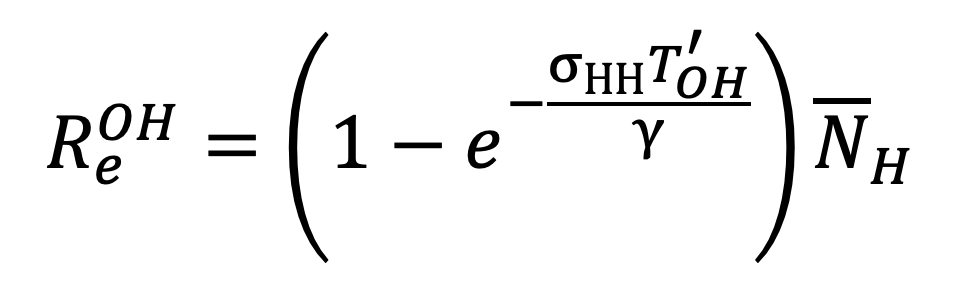
If we assume that infection between residents and visitors to the household happens at the same pairwise transmission rate as infection between members of a shared household, then we can use Equation 14 to estimate an SITP for the other home route of transmission. Denoting this SITP by , we have
|
Equation 15. |
|
where is the expected time per day spent in other households measured by the TUS.
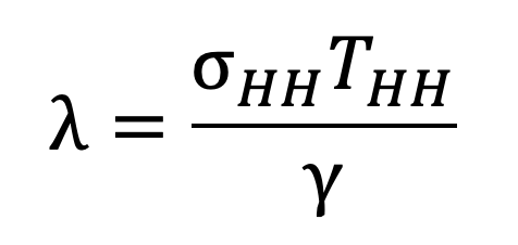
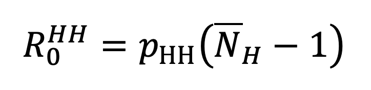
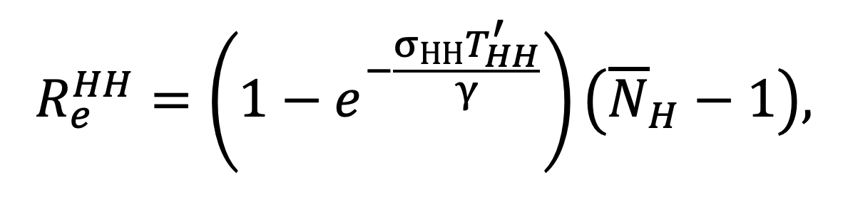
The basic reproductive ratio associated with within-household transmission is given by multiplying the SITP by the expected number of susceptible individuals which the first case in a household will be exposed to during their infectious period. This is precisely the mean household size, , minus one (since the infectious individual cannot transmit to themself). Thus
|
Equation 16. |
|
and analogously
|
Equation 17. |
|
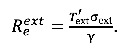
The basic reproductive ratio for external transmission is given by
|
Equation 18. |
|
where is the transmission rate across external social contacts and is the average duration of exposure across all external settings in a single day.
In a real-world outbreak setting, we generally have population-level estimates of which are not subdivided by transmission pathway. Given estimates of the SITP, , and the distribution of household sizes, we can estimate the within-household and other household reproductive ratios using Equations 16 and 17 respectively. Given an estimate of the population-level basic reproductive ratio we can then estimate using equation 10. With this in mind, in our study we modelled the impact of NPIs under a range of values of and to explore the impact of differences in overall transmissibility and the relative contributions of infection within the household and elsewhere.
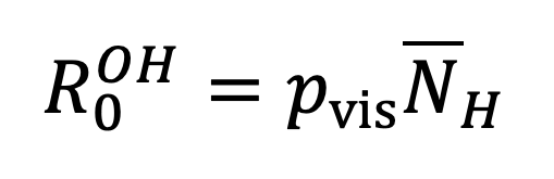
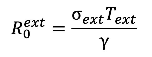
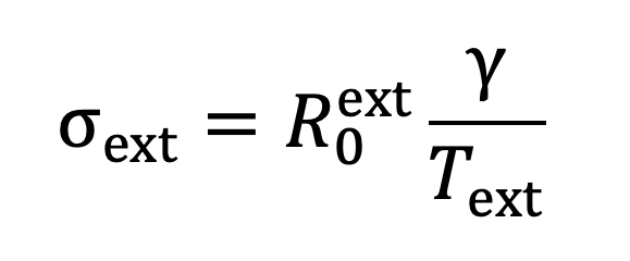
The impact of NPIs is to adjust the average exposure times while keeping transmission rates fixed, as outlined in the section titled ‘Implementation of NPIs’. In the absence of NPIs, we use values estimated from the TUS data: given an estimate of the person-time exposure matrix for transmission pathway , the average daily exposure time associated with this pathway is given by the leading eigenvalue of . The transmission rates across contacts can be estimated from estimates of and by rearranging Equations 16 and 18 as follows:
|
Equation 19. |
|
and
|
Equation 20. |
|
Under an NPI which replaces the exposure times , and with , and respectively, the effective reproductive ratio is given by:
|
Equation 21. |
|
where
|
Equation 22. |
|
|
Equation 23. |
|
and
|
Equation 24. |
|
The TUS data includes estimates of mean enjoyment levels associated with each location category; each survey participant recorded a subjective level of enjoyment on a scale of 1 to 7 during each time interval of the survey day, and the mean enjoyment level for a location is calculated by taking the mean of the recorded enjoyment level over all time intervals associated with that location over all survey participants. These location-specific mean enjoyment levels are stratified by age, so that for each location we can define an age-stratified enjoyment vector . The true impact of NPIs on wellbeing is likely to be difficult to quantify, so to cover a range of possibilities, we model a simple best-case scenario and a simple worst-case scenario, with more complex real-world responses lying somewhere between the two:
All the NPIs we consider in our modelling work by keeping individuals at home when they would otherwise be in some other location, and so we only need to consider changes in subjective enjoyment resulting from increased time at home balanced by decreased time elsewhere.
Denote by the total number of people-minutes recorded by the TUS – 144 times twice the total number of survey participants – and for each location denote the total number of people-minutes spent by people in age group in location in the absence of NPIs as . We define population-level enjoyment to be the sum over all locations and age groups of the total number of person-minutes spent by members of that age group in that location multiplied by the mean enjoyment associated with that age group and location, divided by the total number of people-minutes
|
Equation 25. |
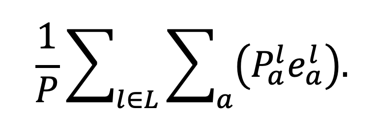
|
If the effect of an NPI is to replace the person-minute profile with , for non-home locations then under the best-case scenario, the total population-level enjoyment is given by
|
Equation 26. |
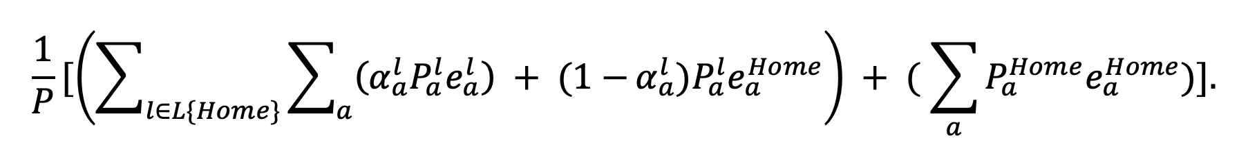
|
The worst-case scenario is calculated as
|
Equation 27. |
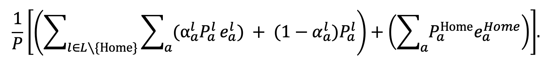
|
Ajelli, M., P. Poletti, A. Melegaro and S. Merler (2014), ‘The role of different social contexts in shaping influenza transmission during the 2009 pandemic’, Scientific Reports, 4 (1), 1–7
Anderson, R., G. Medley, R. May, and A. Johnson, (1986), ‘A preliminary study of the transmission dynamics of the human immunodeficiency virus (HIV), the causative agent of AIDS’, Mathematical Medicine and Biology: A Journal of the IMA, 3 (4), 229–63
Banks, C., E. Colman, T. Doherty, O. Tearne, M. Arnold, K. Atkins, D. Balaz, G. Beaunée, P. Bessell, J. Enright, A. Kleczkowski, G. Rossi, A.-S. Ruget, and R. Kao, (2020), ‘Disentangling the roles of human mobility and deprivation on the transmission dynamics of COVID-19 using a spatially explicit simulation model’, medRxiv, available at: https://www.semanticscholar.org/paper/Disentangling-the-roles-of-human-mobility-and-on-of-Banks-Colman/3e1673b407cf616efaa54533bb47c1778d302f3e
Banks, J. and X. Xu, (2020), ‘The mental health effects of the first two months of lockdown during the COVID-19 pandemic in the UK’, Fiscal Studies, 41 (3), 685–708
Brooks, S. K., R. K. Webster, L. E. Smith, L. Woodland, S. Wessely, N. Greenberg, and G.J. Rubin (2020), ‘The psychological impact of quarantine and how to reduce it: rapid review of the evidence’, The Lancet, 395 (10227), 912–20
Chandola, T., M. Kumari, C. L. Booker, and M. Benzeval (2022), ‘The mental health impact of COVID-19 and lockdown-related stressors among adults in the UK’, Psychological Medicine, 52 (14), 2997–3006
Chang, S., E. Pierson, P. W. Koh, J. Gerardin, B. Redbird, D. Grusky, and J. Leskovec, (2021), ‘Mobility network models of COVID-19 explain inequities and inform reopening’, Nature, 589 (7840), 82–87
Davies, N. G., A.J. Kucharski, R.M. Eggo, A. Gimma, W.J. Edmunds, on behalf of the Centre for the Mathematical Modelling of Infectious Diseases COVID-19 working group (2020), ‘Effects of nonpharmaceutical interventions on COVID-19 cases, deaths, and demand for hospital services in the UK: A modelling study’, The Lancet Public Health, 5 (7), e375–e385
Dimeglio, C., J.-M. Loubes, J.-M. Mansuy, and J. Izopet (2021), ‘Quantifying the impact of public health protection measures on the spread of sars-cov-2’, Journal of Infection, 82 (3), 414– 51
Evans, S., E. Alkan, J. K. Bhangoo, H. Tenenbaum, and T. Ng-Knight (2021), ‘Effects of the COVID-19 lockdown on mental health, wellbeing, sleep, and alcohol use in a UK student sample’, Psychiatry Research, 298, 113819
Eyre, R. W., T. House, E. M. Hill, and F.E. Griffiths (2017), ‘Spreading of components of mood in adolescent social networks’, Royal Society Open Science, 4 (170336)
Fancourt, D., A. Steptoe, and F. Bu (2020), ‘Trajectories of anxiety and depressive symptoms during enforced isolation due to COVID-19: Longitudinal analyses of 36,520 adults in England’, Lancet Psychiatry, 8 (2), 141–49
Firth, J. A., J. Hellewell, P. Klepac, S. Kissler, M. Jit, K. E. Atkins, S. Clifford, C.J. Villabona-Arenas, S.R. Meakin, C. Diamond, N.I. Bosse, J.D. Munday, K. Prem, A. M. Foss, E.S. Nightingale, K. v. Zandvoort, N.G. Davies, H.P. Gibbs, G. Medley, A. Gimma, S. Flasche, D. Simons, M. Auzenbergs, T. W. Russell, B.J. Quilty, E. M. Rees, Q. J. Leclerc, W. J. Edmunds, S. Funk, R. M. G. J. Houben, G. M. Knight, S. Abbott, F. Y. Sun, R. Lowe, D. C. Tully, S. R. Procter, C. I. Jarvis, A. Endo, Y. O’Reilly, K., Emery, J. C., Jombart, T., Rosello, A., Deol, A. K., Quaife, M., Hué, S., Liu, R. M. Eggo, C. A. B. Pearson, A. J. Kucharski, L. G. Spurgin and CMMID COVID-19 Working Group (2020), ‘Using a real-world network to model localized COVID-19 control strategies’, Nature Medicine, 26: 1616–22
Flaxman, S., S. Mishra, A. Gandy, H. J. T. Unwin, T. A. Mellan, H. Coupland, C. Whittaker, H. Zhu, T. Berah, J.W. Eaton, M. Monod, M., P.N Perez-Guzman, Schmit, N., Cilloni, L., Ainslie, K. E. C., Baguelin, M., Boonyasiri, A., Boyd, O., L. Cattarino, L. V. Cooper, Z. Cucunubá, G. Cuomo-Dannenburg, A. Dighe, B. Djaafara, I. Dorigatti, S. L. van Elsland, R. G. FitzJohn, K. A. M. Gaythorpe, L. Geidelberg, N. C. Grassly, W. D. Green, T. Hallett, A. Hamlet, W. Hinsley, B. Jeffrey, E. Knock, D. J. Laydon, G. Nedjati-Gilani, P. Nouvellet, K. V. Parag, I. Siveroni, H. A. Thompson, R. Verity, E. Volz, C. E. Walters, H. Wang, Y. Wang, O. J. Watson, P. Winskill, X. Xi, P. G. T. Walker, A. C. Ghani, C. A. Donnelly, S. Riley, M. A. C. Vollmer, N. M. Ferguson, L. C. Okell, A. Bhatt, and Imperial College COVID-19 Response Team (2020), ‘Estimating the effects of non-pharmaceutical interventions on covid-19 in Europe’, Nature, 584: 257–61
Fumanelli, L., M. Ajelli, P. Manfredi, A. Vespignani, and S. Merler (2012), ‘Inferring the structure of social contacts from demographic data in the analysis of infectious diseases spread’, PLOS Computational Biology doi: 10.1371/journal.pcbi.1002673
Gershuny, J. and O. Sullivan (2017), ‘United Kingdom time use survey, 2014-2015’, Centre for Time Use Research, IOE, University College London. [data collection]. UK Data Service. SN: 8128
Hale, T., N. Angrist, R. Goldszmidt, B. Kira, A. Petherick, T. Phillips, S. Webster, E. Cameron-Blake, L. Hallas, S. Majumdar, H. Tatlow (2021), ‘A global panel database of pandemic policies (Oxford COVID-19 government response tracker)’, Nature Human Behaviour, 5 (4), 529–538
Hilton, J. and M. J. Keeling (2020), ‘Estimation of country-level basic reproductive ratios for novel coronavirus (sars-cov-2/covid-19) using synthetic contact matrices’, PLoS computational biology, 16 (7), e1008031
Hilton, J., H. Riley, L. Pellis, R. Aziza, S. P. C. Brand, S. P. C., I. K. Kombe, J. Ojal, A. Parisi, M. J. Keeling, D. J. Nokes, R. Manson-Sawko, and T. House (2022), ‘A computational framework for modelling infectious disease policy based on age and household structure with applications to the COVID-19 pandemic’, PLOS Computational Biology, 18 (9), 1–38
House, T. and M. J. Keeling (2009), ‘Household structure and infectious disease transmission’, Epidemiology & Infection, 137 (5), 654–61
House, T., H. Riley, L. Pellis, K. B. Pouwels, S. Bacon, A. Eidukas, K. Jahanshahi, R. M. Eggo, and A. Sarah Walker (2022), ‘Inferring risks of coronavirus transmission from community household data’, Statistical Methods in Medical Research, 31 (9), 1738–56.
Jarvis, C. I., K. Van Zandvoort, A. Gimma, K. Prem, P. Klepac, G. J. Rubin, and W. J. Edmunds (2020), ‘Quantifying the impact of physical distance measures on the transmission of covid-19 in the UK’, BMC Medicine, 18 (1), 1–10
Karaivanov, A. (2020), ‘A social network model of COVID-19’, Plos One, 15 (10), e0240878
Keeling, M. J. and K. T. Eames (2005), ‘Networks and epidemic models’, Journal of the Royal Society Interface, 2 (4), 295–307
Keeling, M. and P. Rohani (2007), Modeling Infectious Diseases in Humans and Animals, Princeton, NJ: Princeton University Press
Lai, S., N. W. Ruktanonchai, L. Zhou, O. Prosper, W. Luo, J. R. Floyd, A. Wesolowski, M. Santillana, C. Zhang, X. Du, H. Yu, and A. J. Tatem (2020), ‘Effect of nonpharmaceutical interventions to contain COVID-19 in China’, Nature, 585: 410–13.
Leng, T., E. M. Hill, A. Holmes, E. Southall, R. N. Thompson, M. J. Tildesley, M. J. Keeling, L. and Dyson (2022), ‘Quantifying pupil-to-pupil sars-cov-2 transmission and the impact of lateral flow testing in English secondary schools’, Nature Communications, 13 (1), 1106
Li, Q., X. Guan, P. Wu, X. Wang, L. Zhou, Y. Tong, R. Ren, K. S. Leung, E. H. Lau, J. Y. Wong, X. Xing, N. Xiang, Y. Wu, C. Li, Q. Chen, D. Li, T. Liu, J. Zhao, M. Liu, W. Tu, C. Chen, L. Jin, R. Yang, Q. Wang, S. Zhou, R. Wang, H. Liu, Y. Luo, Y. Liu, G. Shao, H. Li, Z. Tao, Y. Yang, Z. Deng, B. Liu, Z. Ma, Y. Zhang, G. Shi, T. T. Lam, J. T. Wu, G. F. Gao, B. J. Cowling, B. Yang, G. M. Leung, and Z. Feng (2020), ‘Early transmission dynamics in Wuhan, China, of novel coronavirus–infected pneumonia’, New England Journal of Medicine, 382 (13), 1199–1207. PMID: 31995857
Liu, Y., A. A. Gayle, A. Wilder-Smith and J. Rocklöv (2020), ‘The reproductive number of COVID-19 is higher compared to sars coronavirus’, Journal of Travel Medicine, 27 (2), taaa021, doi: 10.1093/jtm/taaa021
Moore, S., E. M. Hill, M. J. Tildesley, L. Dyson and M. J. Keeling (2021), ‘Vaccination and non-pharmaceutical interventions for COVID-19: a mathematical modelling study’, The Lancet Infectious Diseases, 21 (6), 793–802
Mossong, J., N. Hens, M. Jit, P. Beutels, K. Auranen, R. Mikolajczyk, M. Massari, S. Salmaso, G. S. Tomba, J. Wallinga, J. Heijne, M. Sadkowska-Todys, M. Rosinska and W. J. Edmunds (2008), ‘Social contacts and mixing patterns relevant to the spread of infectious diseases’, PLoS medicine, 5 (3), e74
Niedzwiedz, C. L., M. J. Green, M. Benzeval, D. Campbell, P. Craig, E. Demou, A. Leyland, A. Pearce, R. Thomson, E. Whitley, S. V. Katikireddi (2021), ‘Mental health and health behaviours before and during the initial phase of the COVID-19 lockdown: Longitudinal analyses of the UK household longitudinal study’, J Epidemiol Community Health, 75 (3), 224–231
ONS (2024), 'Population estimates for the UK, England, Wales, Scotland, and Northern Ireland - Office for National Statistics 2024.', available at https: //www.ons.gov.uk/peoplepopulationandcommunity/populationandmigration/populationestimates/bulletins/annualmidyearpopulationestimates/mid2022, accessed August 23, 2024)
Owens, M., E. Townsend, E. Hall, T. Bhatia, R. Fitzgibbon, and F. Miller-Lakin (2022), ‘Mental health and wellbeing in young people in the UK during lockdown (COVID-19)’, International Journal of Environmental Research and Public Health, 19 (3), 1132
O’Driscoll, M., G. Ribeiro Dos Santos, L. Wang, D. A. Cummings, A. S. Azman, J. Paireau, A. Fontanet, S. Cauchemez, and H. Salje (2021), ‘Age-specific mortality and immunity patterns of sars-cov-2’, Nature, 590 (7844), 140–45
Pellis, L., N. M. Ferguson, and C. Fraser (2011), ‘Epidemic growth rate and household reproduction number in communities of households, schools and workplaces’, Journal of Mathematical Biology, 63 (4), 691–734
Perra, N. (2021), ‘Non-pharmaceutical interventions during the COVID-19 pandemic: A review’, Physics Reports, 913, 1–52
Prem, K., Y. Liu, T. Russell, A. Kucharski, R. Eggo, N. Davies, M. Jit, P. Klepac, S. Flasche, S. Clifford, C. Pearson, J. Munday, S. Abbott, H. Gibbs, A. Rosello, B. Quilty, T. Jombart, F. Sun, C. Diamond, and J. Hellewell (2020), ‘The effect of control strategies to reduce social mixing on outcomes of the COVID-19 epidemic in Wuhan, China: A modelling study’, The Lancet Public Health, 5
Prem, K., K. van Zandvoort, P. Klepac, R. M. Eggo, N. G. Davies, A. R. Cook, and M. Jit (2021), ‘Projecting contact matrices in 177 geographical regions: An update and comparison with empirical data for the COVID-19 era’, PLoS Computational Biology, 17 (7), 1–19
Ross, J. V., T. House, and M. J. Keeling (2010), ‘Calculation of disease dynamics in a population of households’, PLoS One, 5 (3), e9666
Schenzle, D. (1984), ‘An age-structured model of pre- and post-vaccination measles transmission’, Mathematical Medicine and Biology: A Journal of the IMA, 1 (2), 169–91
Silva, P. J. S., T. Pereira, C. Sagastiz´abal, L. Nonato, M. M. Cordova and C. J. Struchiner (2021), ‘Smart testing and critical care bed sharing for COVID-19 control’, PLOS ONE, 16 (10), 1–17
Stroud, I. and L. M. Gutman (2021), ‘Longitudinal changes in the mental health of UK young male and female adults during the COVID-19 pandemic’, Psychiatry Research, 303: 114074
van Leeuwen, E., P. J. M. Group, and F. Sandmann (2022), ‘Augmenting contact matrices with time-use data for fine-grained intervention modelling of disease dynamics: A modelling analysis’, Statistical Methods in Medical Research, 31 (9), 1704–15
White, R. G. and C. Van Der Boor (2020), ‘Impact of the COVID-19 pandemic and initial period of lockdown on the mental health and well-being of adults in the UK’, BJPsych Open, 6 (5)
Zagheni, E., F. C. Billari, P. Manfredi, A. Melegaro, J. Mossong, and W. J. Edmunds (2008), ‘Using time-use data to parameterize models for the spread of close-contact infectious diseases’, American Journal of Epidemiology, 168 (9), 1082–90
Basic reproductive ratio: Expected number of infections generated by a single infection in a population with no pre-existing immunity and in the absence of control measures.
Contact matrix: A matrix in which the entries quantify the intensity of social contacts relevant to infectious disease transmission between different groups in a population stratified into age or risk classes.
Dynamic model: A mathematical tool used to analyse the evolution of a physical, biological or social process over time.
Effective reproductive ratio: Expected number of infections generated by a single infection in a population during an evolving outbreak of infection, potentially in a partially immune population and with control measures implemented.
Eigenvalue: The scalar multiplier associated with a given eigenvector of an operator.
Lateral flow test: Common testing method which detects antigens that are present when a person has COVID-19.
Matrix: (pl. matrices) A table-like mathematical structure which encodes a specific geometrical transformation in multidimensional space.
Non-pharmaceutical intervention (NPI): Any public health measure that does not primarily use medication, e.g. lockdown.
Pandemic: An outbreak of a disease that effects an entire country, several countries or the whole world at one time.
Poisson Process: A stochastic process in which events occur at a constant rate and independently of one another
Time-use survey: A survey designed to quantitatively study human behaviour by asking participants to record their social activities at different times of day.
To cite this paper please use the following details: Brooks, J. T. (2024), 'Modelling wellbeing during public health interventions for respiratory epidemics', Reinvention: an International Journal of Undergraduate Research, Volume 17, Issue 2, https://reinventionjournal.org/index.php/reinvention/article/view/1488/1367. Date accessed [insert date]. If you cite this article or use it in any teaching or other related activities please let us know by e-mailing us at Reinventionjournal@warwick.ac.uk.